We have already seen the different means that C offers for conditional execution: execution that, based on a value, chooses one branch of the program over another to continue. The reason for a potential “jump” to another part of the program code (for example, to an else branch) is a runtime decision that depends on runtime data. This chapter starts with a discussion of unconditional ways to transfer control to other parts of our code: by themselves, they do not require any runtime data to decide where to go.
The code examples we have seen so far often used functions from the C library that provided features we did not want (or were not able) to implement ourselves, such as printf for printing and strlen for computing the length of a string. The idea behind this concept of functions is that they implement a certain feature, once and for all, and that we then can rely on that feature in the rest of our code.
A function for which we have seen several definitions is main, the entry point of execution into a program. In this chapter, we will look at how to write functions ourselves that may provide features just like the functions in the C library.
The main reasons motivating the concept of functions are modularity and code factorization:
In addition to functions, C has other means of unconditional transfer of control, which are mostly used to handle error conditions or other forms of exceptions from the usual control flow:
We have used a lot of functions and seen some of their declarations (for example in section 6.1.5) and definitions (such as listing 6.3). In all of these functions, parentheses () play an important syntactical role. They are used for function declarations and definitions, to encapsulate the list of parameter declarations. For function calls, they hold the list of arguments for that concrete call. This syntactic role is similar to [] for arrays: in declarations and definitions, they contain the size of the corresponding dimension. In a designation like A[i], they are used to indicate the position of the accessed element in the array.
All the functions we have seen so far have a prototypeC: their declaration and definition, including a parameter type-list and a return type. To see that, let us revisit the leapyear function from listing 6.3:
 5   bool leapyear(unsigned year) {
 6     /* All years that are divisible by 4 are leap years,
 7        unless they start a new century, provided they
 8        are not divisible by 400. */
 9     return !(year % 4) && ((year % 100) || !(year % 400));
10   }
A declaration of that function (without a definition) could look as follows:
bool leapyear(unsigned year);
Alternatively, we could even omit the name of the parameter and/or add the storage specifier extern:[1]
More details on the keyword extern will be provided in section 13.2.
extern bool leapyear(unsigned);
Important for such a declaration is that the compiler sees the types of the argument(s) and the return type, so here the prototype of the function is “function receiving an unsigned and returning a bool."
There are two special conventions that use the keyword void:
Such a prototype helps the compiler in places where the function is to be called. It only has to know about the parameters the function expects. Have a look at the following:
   extern double fbar(double);

   ...
   double fbar2 = fbar(2)/2;
Here, the call fbar(2) is not directly compatible with the expectation of function fbar: it wants a double but receives a signed int. But since the calling code knows this, it can convert the signed int argument 2 to the double value 2.0 before calling the function. The same holds for the use of the return value in an expression: the caller knows that the return type is double, so floating-point division is applied for the result expression.
C has obsolete ways to declare functions without prototype, but you will not see them here. You shouldn’t use them; they will be retired in future versions.
All functions must have prototypes.
A notable exception to that rule are functions that can receive a varying number of parameters, such as printf. They use a mechanism for parameter handling called a variable argument listC, which comes with the header stdargs.h.
<stdargs.h>
We will see later (section 16.5.2) how this works, but this feature is to be avoided in any case. Already from your experience with printf you can imagine why such an interface poses difficulties. You, as the programmer of the calling code, have to ensure consistency by providing the correct "%XX" format specifiers.
In the implementation of a function, we must watch that we provide return values for all functions that have a non-void return type. There can be several return statements in a function:
Functions have only one entry but can have several returns.
All returns in a function must be consistent with the function declaration. For a function that expects a return value, all return statements must contain an expression; functions that expect none, mustn’t contain expressions.
A function return must be consistent with its type.
But the same rule as for the parameters on the calling side holds for the return value. A value with a type that can be converted to the expected return type will be converted before the return happens.
If the type of the function is void, the return (without expression) can even be omitted:
Reaching the end of the {} block of a function is equivalent to a return statement without an expression.
Because otherwise a function that returns a value would have an indeterminate value to return, this construct is only allowed for functions that do not return a value:
Reaching the end of the {} block of a function is only allowed for void functions.
Perhaps you have noted some particularities about main. It has a very special role as the entry point into your program: its prototype is enforced by the C standard, but it is implemented by the programmer. Being such a pivot between the runtime system and the application, main has to obey some special rules.
First, to suit different needs, it has several prototypes, one of which must be implemented. Two should always be possible:
int main(void);
int main(int argc, char* argv[argc+1]);
Then, any C platform may provide other interfaces. Two variations are relatively common:
You should not rely on the existence of such other forms. If you want to write portable code (which you do), stick to the two “official” forms. For these, the return value of int gives an indication to the runtime system if the execution was successful: a value of EXIT_SUCCESS or EXIT_FAILURE indicates success or failure of the execution from the programmer’s point of view. These are the only two values that are guaranteed to work on all platforms.
Use EXIT_SUCCESS and EXIT_FAILURE as return values for main.
In addition, there is a special exception for main, as it is not required to have an explicit return statement:
Reaching the end of main is equivalent to a return with value EXIT_SUCCESS.
Personally, I am not much of a fan of such exceptions without tangible gain; they just make arguments about programs more complicated.
The library function exit has a special relationship with main. As the name indicates, a call to exit terminates the program. The prototype is as follows:
_Noreturn void exit(int status);
This function terminates the program exactly as a return from main would. The status parameter has the role that the return expression in main would have.
Calling exit(s) is equivalent to the evaluation of return s in main.
We also see that the prototype of exit is special because it has a void type. Just like a return statement, exit never fails.
exit never fails and never returns to its caller.
The latter is indicated by the special keyword _Noreturn. This keyword should only be used for such special functions. There is even a pretty-printed version of it, the macro noreturn, which comes with the header stdnoreturn.h.
<stdnoreturn.h>
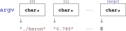
There is another feature in the second prototype of main: argv, the vector of command-line arguments. We looked at some examples where we used this vector to communicate values from the command line to the program. For example, in listing 3.1, these command-line arguments were interpreted as double data for the program:
So each of the argv [i] for i = 0,..., argc is a pointer similar to those we encountered earlier. As an easy first approximation, we can see them as strings.
All command-line arguments are transferred as strings.
It is up to us to interpret them. In the example, we chose the function strtod to decode a double value that was stored in the string.
Of the argv strings, two elements hold special values:
Of the arguments to main, argv[0] holds the name of the program invocation.
There is no strict rule about what program name should be, but usually it is the name of the program executable.
Of the arguments to main, argv[argc] is 0.
In the argv array, the last argument could always be identified using this property, but this feature isn’t very useful: we have argc to process that array.
An important feature of functions is encapsulation: local variables are only visible and alive until we leave the function, either via an explicit return or because execution falls out of the last enclosing brace of the function’s block. Their identifiers (names) don’t conflict with other similar identifiers in other functions, and once we leave the function, all the mess we leave behind is cleaned up.
Even better: whenever we call a function, even one we have called before, a new set of local variables (including function parameters) is created, and these are newly initialized. This also holds if we newly call a function for which another call is still active in the hierarchy of calling functions. A function that directly or indirectly calls itself is called recursive, and the concept is called recursion.
Recursive functions are crucial for understanding C functions: they demonstrate and use primary features of the function call model and are only fully functional with these features. As a first example, we will look at an implementation of Euclid’s algorithm to compute the greatest common divisor (gcd) of two numbers:
 8   size_t gcd2(size_t a, size_t b) {
 9     assert(a <= b);
10     if (!a) return b;
11     size_t rem = b % a;
12     return gcd2(rem, a);
13   }
As you can see, this function is short and seemingly nice. But to understand how it works, we need to thoroughly understand how functions work, and how we transform mathematical statements into algorithms.
Given two integers a, b > 0, the gcd is defined as the greatest integer c > 0 that divides into both a and b. Here is the formula:
 | c|a and c|b}
If we also assume that a < b, we can easily see that two recursive formulas hold:
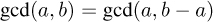
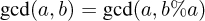
That is, the gcd doesn’t change if we subtract the smaller integer or if we replace the larger of the two with the modulus
of the other. These formulas have been used to compute the gcd since the days of ancient Greek mathematics. They are commonly
attributed to Euclid ( , around 300 B.C.) but may have been known even before him.
Our C function gcd2 uses equation (7.2). First (line 9), it checks if a precondition for the execution of this function is satisfied: whether the first argument is less than or equal to the second. It does this by using the assert macro from assert.h. This would abort the program with an informative message if the function was called with arguments that didn’t satisfy that condition (we will see more explanations of assert in section 8.7).
<assert.h>
Make all preconditions for a function explicit.
Then, line 10 checks whether a is 0, in which case it returns b. This is an important step in a recursive algorithm:
In a recursive function, first check the termination condition.
A missing termination check leads to infinite recursion; the function repeatedly calls new copies of itself until all system resources are exhausted and the program crashes. On modern systems with large amounts of memory, this may take some time, during which the system will be completely unresponsive. You’d better not try it.
Otherwise, we compute the remainder rem of b modulo a (line 11). Then the function is called recursively with rem and a, and the return value of that is directly returned.
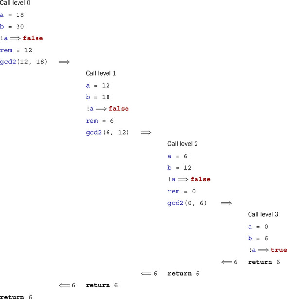
Figure 7.1 shows an example of the different recursive calls that are issued from an initial call gcd2(18, 30). Here, the recursion goes four levels deep. Each level implements its own copies of the variables a, b, and rem.
For each recursive call, modulo arithmetic (takeaway 4.8) guarantees that the precondition is always fulfilled automatically. For the initial call, we have to ensure this ourselves. This is best done by using a different function, a wrapperC:
15   size_t gcd(size_t a, size_t b) {
16     assert(a);
17     assert(b);
18     if (a < b)
19       return gcd2(a, b);
20     else
21       return gcd2(b, a);
22   }
Ensure the preconditions of a recursive function in a wrapper function.
This avoids having to check the precondition at each recursive call: the assert macro is such that it can be disabled in the final production object file.
Another famous example of a recursive definition of an integer sequence are Fibonnacci numbers, a sequence of numbers that appeared as early as 200 B.C. in Indian texts. In modern terms, the sequence can be defined as


The sequence of Fibonacci numbers is fast-growing. Its first elements are 1, 1, 2, 3, 5, 8, 13, 21, 34, 55, 89, 144, 377, 610, 987.
With the golden ratio
it can be shown that
and so, asymptotically, we have

So the growth of Fn is exponential.
The recursive mathematical definition can be translated in a straightforward manner into a C function:
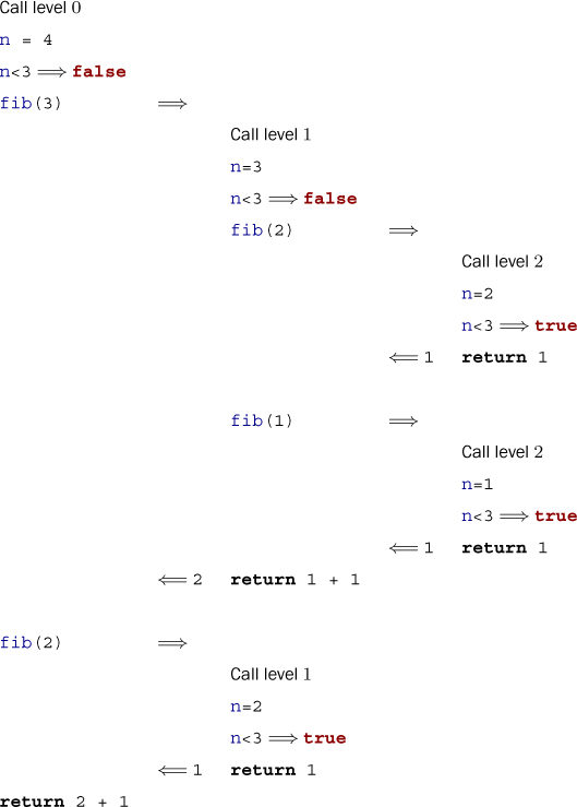
4   size_t fib(size_t n) {
5     if (n < 3)
6       return 1;
7     else
8       return fib(n-1) + fib(n-2);
9   }
Here, again, we first check for the termination condition: whether the argument to the call, n, is less than 3. If it is, the return value is 1; otherwise we return the sum of calls with argument values n-1 and n-2.
Figure 7.2 shows an example of a call to fib with a small argument value. We see that this leads to three levels of stacked calls to the same function with different arguments. Because equation (7.5) uses two different values of the sequence, the scheme of the recursive calls is much more involved than the one for gcd2. In particular, there are three leaf calls: calls to the function that fulfill the termination condition, and thus by themselves not go into recursion.[[Exs 1]]
Show that a call fib(n) induces Fn leaf calls.
Implemented like that, the computation of the Fibonacci numbers is quite slow.[[Exs 2]] In fact, it is easy to see that the recursive formula for the function itself also leads to an analogous formula for the function’s execution time:
Measure the times for calls to fib(n) with n set to different values. On POSIX systems, you can use /bin/time to measure the run time of a program’s execution.
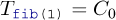

where C0 and C1 are constants that depend on the platform.
It follows that regardless of the platform and the cleverness of our implementation, the function’s execution time will always be something like
with another platform-dependent constant C2. So the execution time of fib(n) is exponential in n, which usually rules out using such a function in practice.
Multiple recursion may lead to exponential computation times.
If we look at the nested calls in figure 7.2, we see that we have the call fib(2) twice, and thus all the effort to compute the value for fib(2) is repeated. The following fibCacheRec function avoids such repetitions. It receives an additional argument, cache, which is an array that holds all values that have already been computed:
 4   /* Compute Fibonacci number n with the help of a cache that may
 5      hold previously computed values. */
 6   size_t fibCacheRec(size_t n, size_t cache[n]) {
 7     if (!cache[n-1]) {
 8       cache[n-1]
 9         = fibCacheRec(n-1, cache) + fibCacheRec(n-2, cache);
10     }
11     return cache[n-1];
12   }
13
14   size_t fibCache(size_t n) {
15     if (n+1 <= 3) return 1;
16     /* Set up a VLA to cache the values. */
17     size_t cache[n];
18     /* A VLA must be initialized by assignment. */
19     cache[0] = 1; cache[1] = 1;
20     for (size_t i = 2; i < n; ++i)
21       cache[i] = 0;
22     /* Call the recursive function. */
23     return fibCacheRec(n, cache);
24   }
By trading storage against computation time, the recursive calls are affected only if the value has not yet been computed. Thus the fibCache(i) call has an execution time that is linear in n
for a platform-dependent parameter C3.[[Exs 3]] Just by changing the algorithm that implements our sequence, we are able to reduce the execution time from exponential to linear! We didn’t (and wouldn’t) discuss implementation details, nor did we perform concrete measurements of execution time.[[Exs 4]]
Prove equation (7.13).
Measure times for fibCache (n) call with the same values as for fib.
A bad algorithm will never lead to a implementation that performs well.
Improving an algorithm can dramatically improve performance.
For the fun of it, fib2Rec shows a third implemented algorithm for the Fibonacci sequence. It gets away with a fixed-length array (FLA) instead of a variable-length array (VLA).
 4   void fib2rec(size_t n, size_t buf[2]) {
 5     if (n > 2) {
 6       size_t res = buf[0] + buf[1];
 7       buf[1] = buf[0];
 8       buf[0] = res;
 9       fib2rec(n-1, buf);
10     }
11   }
12
13   size_t fib2(size_t n) {
14     size_t res[2] = { 1, 1, };
15     fib2rec(n, res);
16     return res[0];
17   }
Proving that this version is still correct is left as an exercise.[[Exs 5]] Also, up to now we have only had rudimentary tools to assess whether this is “faster” in any sense we might want to give the term.[[Exs 6]]
Use an iteration statement to transform fib2rec into a nonrecursive function fib2iter.
Measure times for fib2(n) calls with the same values as fib.
Now that we’ve covered functions, see if you can implement a program factor that receives a number N on the command line and prints out
N: F0 F1 F2 ...
where F0 and so on are all the prime factors of N.
The core of your implementation should be a function that, given a value of type size_t, returns its smallest prime factor.
Extend this program to receive a list of such numbers and output such a line for each of them.