This chapter covers
Once you feel more comfortable when coding in C, you will perhaps be tempted to do complicated things to “optimize” your code. Whatever you think you are optimizing, there is a good chance you will get it wrong: premature optimization can do a great deal of harm in terms of readability, soundness, maintainability, and so on. Knuth [1974] coined the following phrase that should be your motto for this whole level:
Premature optimization is the root of all evil.
Its good performance is often cited as one of the main reasons C is used so widely. While there is some truth to the idea that many C programs outperform code of similar complexity written in other programming languages, this aspect of C may come with a substantial cost, especially concerning safety. This is because C, in many places, doesn’t enforce rules, but places the burden of verifying them on the programmer. Important examples for such cases are
These can result in program crashes, loss of data, incorrect results, exposure of sensitive information, and even loss of money or lives.
Do not trade off safety for performance.
C compilers have become much better in recent years; basically, they complain about all problems that are detectable at compile time. But severe problems in code can still remain undetected in code that tries to be clever. Many of these problems are avoidable, or at least detectable, by very simple means:
void func(double a[static 1]);
void func(double a[static 7]);
void func(size_t n, double a[n]);
void func(double * a);
Despite what some urban myths suggest, applying these rules usually will not negatively impact the performance of your code.
Optimizers are clever enough to eliminate unused initializations.
The different notations of pointer arguments to functions result in the same binary code.
Not taking addresses of local variables helps the optimizer because it inhibits aliasing.
Once we have applied these rules and have ensured that our implementation is safe, we may have a look at the performance of the program. What constitutes good performance and how we measure it is a difficult subject by itself. A first question concerning performance should always be relevance: for example, improving the runtime of an interactive program from 1 ms to 0.9 ms usually makes no sense at all, and any effort spent making such an improvement is probably better invested elsewhere.
To equip us with the necessary tools to assess performance bottlenecks, we will discuss how to measure performance (section 15.3). This discussion comes at the end of this chapter because before we can fully understand measuring performance, we have to better understand the tools for making performance improvements.
There are many situations in which we can help our compiler (and future versions of it) to optimize code better, because we can specify certain properties of our code that it can’t deduce automatically. C introduces keywords for this purpose that are quite special in the sense that they constrain not the compiler but the programmer. They all have the property that removing them from valid code where they are present should not change the semantics. Because of that property, they are sometimes presented as useless or even obsolete features. Be careful when you encounter such statements: people who make such claims tend not to have a deep understanding of C, its memory model, or its optimization possibilities. And, in particular, they don’t seem to have a deep understanding of cause and effect, either.
The keywords that introduce these optimization opportunities are register (C90), inline, restrict (both from C99), and alignas (respectively _Alignas, C11). As indicated, all four have the property that they could be omitted from a valid program without changing its semantics.
In section 13.2, we spoken to some extent about register, so we will not go into more detail than that. Just remember that it can help to avoid aliasing between objects that are defined locally in a function. As stated there, I think this is a feature that is much underestimated in the C community. I have even proposed ideas to the C committee (Gustedt [2016]) about how this feature could be at the heart of a future improvement of C that would include global constants of any object type and even more optimization opportunities for small pure functions.
In section 12.7, we also discussed C11’s alignas and the related alignof. They can help to position objects on cache boundaries and thus improve memory access. We will not go into more detail about this specialized feature.
The remaining two features, C99’s inline (section 15.1) and restrict (section 15.2), have very different usability. The first is relatively easy to use and presents no danger. It is a tool that is quite widely used and may ensure that the code for short functions can be directly integrated and optimized at the caller side of the function.
The latter, restrict, relaxes the type-based aliasing considerations to allow for better optimization. Thus it is subtle to use and can do considerable harm if used badly. It is often found in library interfaces, but much less in user code.
The remainder of this chapter (section 15.3) dives into performance measurement and code inspection, to enables us to asses performance by itself and the reasons that lead to good or bad performance.
For C programs, the standard tool to write modular code is functions. As we have seen, they have several advantages:
Unfortunately, functions also have some downsides from a performance point of view:
If, by coincidence, the code of the caller (say, fcaller) and the callee (say, fsmall) are present inside the same translation unit (TU), a good compiler may avoid these downsides by inlining. Here, the compiler does something equivalent to replacing the call to fsmall with the code of fsmall itself. Then there is no call, and so there is no call overhead.
Even better, since the code of fsmall is now inlined, all instructions of fsmall are seen in that new context. The compiler can detect, for example,
Inlining can open up a lot of optimization opportunities.
A traditional C compiler can only inline functions for which it also knows the definition: only knowing the declaration is not enough. Therefore, programmers and compiler builders have studied the possibilities to increase inlining by making function definitions visible. Without additional support from the language, there are two strategies to do so:
Where the first approach is infeasible for large projects, the second approach is relatively easy to put in place. Nevertheless, it has drawbacks:
To avoid these drawbacks, C99 has introduced the inline keyword. Unlike what the naming might suggest, this does not force a function to be inlined, but only provides a way that it may be.
The latter point is generally an advantage, but it has one simple problem: no symbol for the function would ever be emitted, even for programs that might need such a symbol. There are several common situations in which a symbol is needed:
To provide such a symbol, C99 has introduced a special rule for inline functions.
Adding a compatible declaration without the inlinekeyword ensures the emission of the function symbol in the current TU.
As an example, suppose we have an inline function like this in a header file: say toto.h:
 1   // Inline definition in a header file.
 2   // Function argument names and local variables are visible
 3   // to the preprocessor and must be handled with care.
 4   inline
 5   toto* toto_init(toto* toto_x) {
 6     if (toto_x) {
 7       *toto_x = (toto){ 0 };
 8     }
 9     return  toto_x;
10   }
Such a function is a perfect candidate for inlining. It is really small, and the initialization of any variable of type toto is probably best made in place. The call overhead is of the same order as the inner part of the function, and in many cases the caller of the function may even omit the test for the if.
An inlinefunction definition is visible in all TUs.
This function may be inlined by the compiler in all TUs that see this code, but none of them would effectively emit the symbol toto_init. But we can (and should) enforce the emission in one TU, toto.c, say, by adding a line like the following:
1   #include "toto.h"
2
3   // Instantiate in exactly one TU.
4   // The parameter name is omitted to avoid macro replacement.
5   toto* toto_init(toto*);
An inline definition goes in a header file.
An additional declaration without inlinegoes in exactly one TU.
As we said, that mechanism of inline functions is there to help the compiler make the decision whether to effectively inline a function. In most cases, the heuristics that compiler builders have implemented to make that decision are completely appropriate, and you can’t do better. They know the particular platform for which the compilation is done much better than you: maybe this platform didn’t even exist when you wrote your code. So they are in a much better position to compare the trade-offs between the different possibilities.
An important family of functions that may benefit from inline definitions is pure functions, which we met in section 10.2.2. If we look at the example of the rat structure (listing 10.1), we see that all the functions implicitly copy the function arguments and the return value. If we rewrite all these functions as inline in the header file, all these copies can be avoided using an optimizing compiler.[[Exs 1]] [[Exs 2]]
Rewrite the examples from section 10.2.2 with inline.
Revisit the function examples in section 7, and argue for each of them whether they should be defined inline.
So inline functions can be a precious tool to build portable code that shows good performance; we just help the compiler(s) to make the appropriate decision. Unfortunately, using inline functions also has drawbacks that should be taken into account for our design.
First, 15.7 implies that any change you make to an inline function will trigger a complete rebuild of your project and all of its users.
Only expose functions as inlineif you consider them to be stable.
Second, the global visibility of the function definition also has the effect that local identifiers of the function (parameters or local variables) may be subject to macro expansion for macros that we don’t even know about. In the example, we used the toto_ prefix to protect the function parameters from expansion by macros from other include files.
All identifiers that are local to an inlinefunction should be protected by a convenient naming convention.
Third, other than conventional function definitions, inline functions have no particular TU with which they are associated. Whereas a conventional function can access state and functions that are local to the TU (static variables and functions), for an inline function, it would not be clear which copy of which TU these refer to.
inlinefunctions can’t access identifiers of staticfunctions.
inlinefunctions can’t define or access identifiers of modifiable static objects.
Here, the emphasis is on the fact that access is restricted to the identifiers and not the objects or functions themselves. There is no problem with passing a pointer to a static object or a function to an inline function.
We have seen many examples of C library functions that use the keyword restrict to qualify pointers, and we also have used this qualification for our own functions. The basic idea of restrict is relatively simple: it tells the compiler that the pointer in question is the only access to the object it points to. Thus the compiler can make the assumption that changes to the object can only occur through that same pointer, and the object cannot change inadvertently. In other words, with restrict, we are telling the compiler that the object does not alias any other object the compiler handles in this part of the code.
A restrict-qualified pointer has to provide exclusive access.
As is often the case in C, such a declaration places the burden of verifying this property on the caller.
A restrict-qualification constrains the caller of a function.
Consider, for example, the differences between memcpy and memmove:
1   void* memcpy(void*restrict s1, void const*restrict s2,  size_t n);
2   void* memmove(void* s1, const void* s2, size_t n);
For memcpy, both pointers are restrict-qualified. So for the execution of this function, the access through both pointers has to be exclusive. Not only that, s1 and s2 must have different values, and neither of them can provide access to parts of the object of the other. In other words, the two objects that memcpy “sees” through the two pointers must not overlap. Assuming this can help to optimize the function.
In contrast, memmove does not make such an assumption. So s1 and s2 may be equal, or the objects may overlap. The function must be able to cope with that situation. Therefore it might be less efficient, but it is more general.
We saw in section 12.3 that it might be important for the compiler to decide whether two pointers may in fact point to the same object (aliasing). Pointers to different base types are not supposed to alias, unless one of them is a character type. So both parameters of fputs are declared with restrict
1 int fputs(const char *restrict s, FILE *restrict stream);
although it might seem very unlikely that anyone might call fputs with the same pointer value for both parameters.
This specification is more important for functions like printf and friends:
1   int printf(const char *restrict format, ...);
2   int fprintf(FILE *restrict stream, const char *restrict format, ...);
The format parameter shouldn’t alias any of the arguments that might be passed to the ... part. For example, the following code has undefined behavior:
1   char const* format = "format printing itself: %s\n";
2   printf(format, format);   // Restrict violation
This example will probably still do what you think it does. If you abuse the stream parameter, your program might explode:
1   char const* format = "First two bytes in stdin object: %.2s\n";
2   char const* bytes = (char*)stdin; // Legal cast to char
3   fprintf(stdin, format, bytes);    // Restrict violation
Sure, code like this is not very likely to occur in real life. But keep in mind that character types have special rules concerning aliasing, and therefore all string-processing functions may be subject to missed optimization. You could add restrict-qualifications in many places where string parameters are involved, and which you know are accessed exclusively through the pointer in question.
We have several times spoken about the performance of programs without yet talking about methods to assess it. And indeed, we humans are notoriously bad at predicting the performance of code. So, our prime directive for questions concerning performance should be:
Don’t speculate about the performance of code; verify it rigorously.
The first step when we dive into a code project that may be performance-critical will always be to choose the best algorithms that solve the problem(s) at hand. This should be done even before coding starts, so we have to make a first complexity assessment by arguing (but not speculating!) about the behavior of such an algorithm.
Complexity assessment of algorithms requires proofs.
Unfortunately, a discussion of complexity proofs is far beyond the scope of this book, so we will not be able to go into it. But, fortunately, many other books have been written about it. The interested reader may refer to the textbook of Cormen et al. [2001] or to Knuth’s treasure trove.
Performance assessment of code requires measurement.
Measurement in experimental sciences is a difficult subject, and obviously we can’t tackle it here in full detail. But we should first be aware that the act of measuring modifies the observed. This holds in physics, where measuring the mass of an object necessarily displaces it; in biology, where collecting samples of species actually kills animals or plants; and in sociology, where asking for gender or immigration background before a test changes the behavior of the test subjects. Not surprisingly it also holds in computer science and, in particular, for time measurement, since all such time measurements need time themselves to be accomplished.
All measurements introduce bias.
At the worst, the impact of time measurements can go beyond the additional time spent making the measurement. In the first place, a call to timespec_get, for example, is a call to a function that wouldn’t be there if we didn’t measure. The compiler has to take some precautions before any such call, in particular saving hardware registers, and has to drop some assumptions about the state of the execution. So time measurement can suppress optimization opportunities. Also, such a function call usually translates into a system call (a call into the operating system), and this can have effects on many properties of the program execution, such as on the process or task scheduling, or can invalidate data caches.
Instrumentation changes compile-time and runtime properties.
The art of experimental sciences is to address these issues and to ensure that the bias introduced by the measurement is small and so the result of an experiment can be assessed qualitatively. Concretely, before we can do any time measurements on code that interests us, we have to assess the bias that time measurements themselves introduce. A general strategy to reduce the bias of measurement is to repeat an experiment several times and collect statistics about the outcomes. Most commonly used statistics in this context are simple. They concern the number of experiments and their mean value (or average), and also their standard deviation and sometimes their skew.
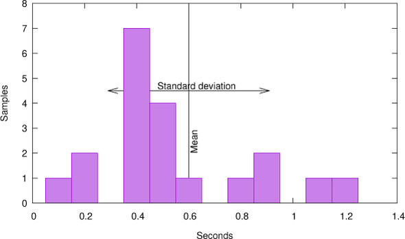
Let us look at the following sample S that consists of 20 timings, in seconds s:
See figure 15.1 for a frequency histogram of this sample. The values show quite a variation
around 0.6 (μ(S), mean value), from 0.1 (minimum) to 1.3 (maximum). In fact, this variation is so important that I personally would not dare to claim much about the relevance of such a sample. These fictive measurements are bad, but how bad are they?
The standard deviation σ(S) measures (again, in seconds) how an observed sample deviates from an ideal world where all timings have exactly the same result. A small standard deviation indicates that there is a good chance the phenomenon that we are observing follows that ideal. Conversely, if the standard deviation is too high, the phenomenon may not have that ideal property (there is something that perturbs our computation), or our measurements might by unreliable (there is something that perturbs our measurement), or both.
For our example, the standard deviation is 0.31, which is substantial compared to the mean value of 0.6: the relative standard deviation σ(S)/μ(S) here is 0.52 (or 52%). Only a value in a low percentage range can be considered good.
The relative standard deviation of run times must be in a low percentage range.
The last statistical quantity that we might be interested in is the skew (0.79 for our sample S). It measures the lopsidedness (or asymmetry) of the sample. A sample that is distributed symmetrically around the mean would have a skew of 0, and a positive value indicates that there is a “tail” to the right. Time measurements usually are not symmetric. We can easily see that in our sample: the maximum value 1.3 is at distance 0.7 from the mean. So for the sample to be symmetric around the mean of 0.6, we would need one value of -0.1, which is not possible.
If you are not familiar with these very basic statistical concepts, you should probably revisit them a bit, now. In this chapter, we will see that all these statistical quantities that interest us can be computed with the raw moments:
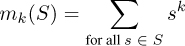
So, the zeroth raw moment counts the number of samples, the first adds up the total number of values, the second is the sum of the squares of the values, and so on.
For computer science, the repetition of an experiment can easily be automated by putting the code that is to be sampled inside a for loop and placing the measurements before and after this loop. Thereby, we can execute the sample code thousands or millions of times and compute the average time spent for a loop iteration. The hope then is that the time measurement can be neglected because the overall time spent in the experiment is maybe several seconds, whereas the time measurement itself may take just several milliseconds.
In this chapter’s example code, we will try to assess the performance of calls to timespec_get and also of a small utility that collects statistics of measurements. Listing 15.1 contains several for loops around different versions of code that we want to investigate. The time measurements are collected in a statistic and use a tv_nsec value obtained from timespec_get. In this approach, the experimental bias that we introduce is obvious: we use a call to timespec_get to measure its own performance. But this bias is easily mastered: augmenting the number of iterations reduces the bias. The experiments that we report here were performed with a value of iterations of 224 – 1.
53      timespec_get(&t[0], TIME_UTC);
54      /* Volatile for i ensures that the loop is effected */
55      for (uint64_t volatile i = 0; i < iterations; ++i) {
56        /* do nothing */
57      }
58      timespec_get(&t[1], TIME_UTC);
59      /* s must be volatile to ensure that the loop is effected */
60      for (uint64_t i = 0; i < iterations; ++i) {
61        s = i;
62      }
63      timespec_get(&t[2], TIME_UTC);
64      /* Opaque computation ensures that the loop is effected */
65      for (uint64_t i = 1; accu0 < upper; i += 2) {
66        accu0 += i;
67      }
68      timespec_get(&t[3], TIME_UTC);
69      /* A function call can usually not be optimized out. */
70      for (uint64_t i = 0; i < iterations; ++i) {
71        timespec_get(&tdummy, TIME_UTC);
72        accu1 += tdummy.tv_nsec;
73      }
74      timespec_get(&t[4], TIME_UTC);
75      /* A function call can usually not be optimized out, but
76         an inline function can. */
77      for (uint64_t i = 0; i < iterations; ++i) {
78        timespec_get(&tdummy, TIME_UTC);
79        stats_collect1(&sdummy[1], tdummy.tv_nsec);
80      }
81      timespec_get(&t[5], TIME_UTC);
82      for (uint64_t i = 0; i < iterations; ++i) {
83        timespec_get(&tdummy, TIME_UTC);
84        stats_collect2(&sdummy[2], tdummy.tv_nsec);
85      }
86      timespec_get(&t[6], TIME_UTC);
87      for (uint64_t i = 0; i < iterations; ++i) {
88        timespec_get(&tdummy, TIME_UTC);
89        stats_collect3(&sdummy[3], tdummy.tv_nsec);
90      }
91      timespec_get(&t[7], TIME_UTC);
But this mostly trivial observation is not the goal; it only serves as an example of some code that we want to measure. The for loops in listing 15.1 contain code that does the statistics collection with more sophistication. The goal is to be able to assert, step by step, how this increasing sophistication influences the timing.
struct timespec tdummy;
stats sdummy[4] = { 0 };
The loop starting on line 70 just accumulates the values, so we may determine their average. The next loop (line 77) uses a function stats_collect1 that maintains a running mean: that is, it implements a formula that computes a new average μn by modifying the previous one by δ(xn, μn–1), where xn is the new measurement and μn–1 is the previous average. The other two loops (lines 82 and 87) then use the functions stats_collect2 and stats_collect3, respectively, which use similar formulas for the second and third moment, respectively, to compute variance and skew. We will discuss these functions shortly.
But first, let us have a look at the tools we use for the instrumentation of the code.
102      for (unsigned i = 0; i < loops; i++) {
103        double diff = timespec_diff(&t[i+1], &t[i]);
104         stats_collect2(&statistic[i], diff);
105      }
We use timespec_diff from section 11.2 to compute the time difference between two measurements and stats_collect2 to sum up the statistics. The whole is then wrapped in another loop (not shown) that repeats that experiment 10 times. After finishing that loop, we use functions for the stats type to print out the result.
109     for (unsigned i = 0; i < loops; i++) {
110       double mean = stats_mean(&statistic[i]);
111       double rsdev  = stats_rsdev_unbiased(&statistic[i]);
112       printf("loop %u: E(t) (sec):\t%5.2e ± %4.02f%%,\tloop body %5.2e\n",
113              i, mean, 100.0*rsdev, mean/iterations);
114     }
Here, obviously, stats_mean gives access to the mean value of the measurements. The function stats_rsdev_unbiased returns the unbiased relative standard deviation: that is, a standard deviation that is unbiased[1] and that is normalized with the mean value.
Such that it is a true estimation of the standard deviation of the expected time, not only of our arbitrary sample.
A typical output of that on my laptop looks like the following:
0     loop 0: E(t) (sec): 3.31e-02 ± 7.30%,  loop body 1.97e-09
1     loop 1: E(t) (sec): 6.15e-03 ± 12.42%, loop body 3.66e-10
2     loop 2: E(t) (sec): 5.78e-03 ± 10.71%, loop body 3.45e-10
3     loop 3: E(t) (sec): 2.98e-01 ± 0.85%,  loop body 1.77e-08
4     loop 4: E(t) (sec): 4.40e-01 ± 0.15%,  loop body 2.62e-08
5     loop 5: E(t) (sec): 4.86e-01 ± 0.17%,  loop body 2.90e-08
6     loop 6: E(t) (sec): 5.32e-01 ± 0.13%,  loop body 3.17e-08
Here, lines 0, 1, and 2 correspond to loops that we have not discussed yet, and lines 3 to 6 correspond to the loops we have discussed. Their relative standard deviations are less than 1%, so we can assert that we have a good statistic and that the times on the right are good estimates of the cost per iteration. For example, on my 2.1 GHz laptop, this means the execution of one loop iteration of loops 3, 4, 5, or 6 takes about 36, 55, 61, and 67 clock cycles, respectively. So the extra cost when replacing the simple sum by stats_collect1 is 19 cycles, from there to stats_collect2 is 6, and yet another 6 cycles are needed if we use stats_collect3 instead.
To see that this is plausible, let us look at the stats type:
1   typedef struct stats stats;
2   struct stats {
3     double moment[4];
4   };
Here we reserve one double for all statistical moments. Function stats_collect in the following listing then shows how these are updated when we collect a new value that we insert.
120   /**
121    ** @brief Add value @a val to the statistic @a c.
122    **/
123   inline
124   void stats_collect(stats* c, double val, unsigned moments) {
125     double n  = stats_samples(c);
126     double n0 = n-1;
127     double n1 = n+1;
128     double delta0 = 1;
129     double delta  = val - stats_mean(c);
130     double delta1 = delta/n1;
131     double delta2 = delta1*delta*n;
132     switch (moments) {
133     default:
134       c->moment[3] += (delta2*n0 - 3*c->moment[2])*delta1;
135     case 2:
136       c->moment[2] += delta2;
137     case 1:
138       c->moment[1] += delta1;
139     case 0:
140       c->moment[0] += delta0;
141     }
142   }
As previously mentioned, we see that this is a relatively simple algorithm to update the moments incrementally. Important features compared to a naive approach are that we avoid numerical imprecision by using the difference from the current estimation of the mean value, and that this can be done without storing all the samples. This approach was first described for mean and variance (first and second moments) by Welford [1962] and was then generalized to higher moments; see Pébay [2008]. In fact, our functions stats_collect1 and so on are just instantiations of that for the chosen number of moments.
154   inline
155   void stats_collect2(stats* c, double val) {
156      stats_collect(c, val, 2);
157   }
The assembler listing in stats_collect2 shows that our finding of using 25 cycles for this functions seems plausible. It corresponds to a handful of arithmetic instructions, loads, and stores.[2]
This assembler shows x86_64 assembler features that we have not yet seen: floating-point hardware registers and instructions, and SSE registers and instructions. Here, memory locations (%rdi), 8(%rdi), and 16(%rdi) correspond to c->moment[i], for i = 0, 1, 2, the name of the instruction minus the v-prefix; sd-postfix shows the operation that is performed; and vfmadd213sd is a floating-point multiply add instruction.
      vmovsd 8(%rdi), %xmm1
      vmovsd (%rdi), %xmm2
      vaddsd .LC2(%rip), %xmm2, %xmm3
      vsubsd %xmm1, %xmm0, %xmm0
      vmovsd %xmm3, (%rdi)
      vdivsd %xmm3, %xmm0, %xmm4
      vmulsd %xmm4, %xmm0, %xmm0
      vaddsd %xmm4, %xmm1, %xmm1
      vfmadd213sd 16(%rdi), %xmm2, %xmm0
      vmovsd %xmm1, 8(%rdi)
      vmovsd %xmm0, 16(%rdi)
Now, by using the example measurements, we still made one systematic error. We took the points of measure outside the for loops. By doing so, our measurements also form the instructions that correspond to the loops themselves. Listing 15.6 shows the three loops that we skipped in the earlier discussion. These are basically empty, in an attempt to measure the contribution of such a loop.
53      timespec_get(&t[0], TIME_UTC);
54      /* Volatile for i ensures that the loop is effected */
55      for (uint64_t volatile i = 0; i < iterations; ++i) {
56        /* do nothing */
57      }
58      timespec_get(&t[1], TIME_UTC);
59      /* s must be volatile to ensure that the loop is effected */
60      for (uint64_t i = 0; i < iterations; ++i) {
61        s = i;
62      }
63      timespec_get(&t[2], TIME_UTC);
64      /* Opaque computation ensures that the loop is effected */
65      for (uint64_t i = 1; accu0 < upper; i += 2) {
66        accu0 += i;
67      }
68      timespec_get(&t[3], TIME_UTC);
In fact, when trying to measure for loops with no inner statement, we face a severe problem: an empty loop with no effect can and will be eliminated at compile time by the optimizer. Under normal production conditions, this is a good thing; but here, when we want to measure, this is annoying. Therefore, we show three variants of loops that should not be optimized out. The first declares the loop variable as volatile such that all operations on the variable must be emitted by the compiler. Listings 15.7 and 15.8 show GCC’s and Clang’s versions of this loop. We see that to comply with the volatile qualification of the loop variable, both have to issue several load and store instructions.
.L510:
        movq 24(%rsp), %rax
        addq $1, %rax
        movq %rax, 24(%rsp)
        movq 24(%rsp), %rax
        cmpq %rax, %r12
        ja .L510
.LBB9_17:
        incq 24(%rsp)
        movq 24(%rsp), %rax
        cmpq %r14, %rax
        jb .LBB9_17
For the next loop, we try to be a bit more economical by only forcing one volatile store to an auxiliary variable s. As we can see in listings 15.9, the result is assembler code that looks quite efficient: it consists of four instructions, an addition, a comparison, a jump, and a store.
.L509:
        movq %rax, s(%rip)
        addq $1, %rax
        cmpq %rax, %r12
        jne .L509
To come even closer to the loop of the real measurements, in the next loop we use a trick: we perform index computations and comparisons for which the result is meant to be opaque to the compiler. Listing 15.10 shows that this results in assembler code similar to the previous, only now we have a second addition instead of the store operation.
.L500:
        addq %rax, %rbx
        addq $2, %rax
        cmpq %rbx, %r13
        ja .L500
Table 15.1 summarizes the results we collected here and relates the differences between the various measurements. As we might expect, we see that loop 1 with the volatile store is 80% faster than the loop with a volatile loop counter. So, using a volatile loop counter is not a good idea, because it can deteriorate the measurement.
On the other hand, moving from loop 1 to loop 2 has a not-very-pronounced impact. The 6% gain that we see is smaller than the standard deviation of the test, so we can’t even be sure there is a gain at all. If we would really like to know whether there is a difference, we would have to do more tests and hope that the standard deviation was narrowed down.
But for our goal to assess the time implications of our observation, the measurements are quite conclusive. Versions 1 and 2 of the for loop have an impact that is about one to two orders of magnitude below the impact of calls to timespec_get or stats_collect. So we can assume that the values we see for loops 3 to 6 are good estimators for the expected time of the measured functions.
There is a strong platform-dependent component in these measurements: time measurement with timespec_get. In fact, we learned from this experience that on my machine,[3] time measurement and statistics collection have a cost that is of the same order of magnitude. For me, personally, this was a surprising discovery: when I wrote this chapter, I thought time measurement would be much more expensive.
A commodity Linux laptop with a recent system and modern compilers as of 2016.
We also learned that simple statistics such as the standard deviation are easy to obtain and can help to assert claims about performance differences.
Collecting higher-order moments of measurements to compute variance and skew is simple and cheap.
So, whenever you make performance claims in the future or see such claims made by others, be sure the variability of the results has at least been addressed.
Runtime measurements must be hardened with statistics.
|
Loop |
Sec per iteration |
Difference |
Gain/loss |
Conclusive |
|
|---|---|---|---|---|---|
| 0 | volatile loop | 1.97 10–09 | |||
| 1 | volatile store | 3.66 10–10 | -1.60 10 –09 | -81% | Yes |
| 2 | Opaque addition | 3.45 10–10 | -2.10 10–11 | -6% | No |
| 3 | Plus timespec_get | 1.77 10–08 | 1.74 10–08 | +5043% | Yes |
| 4 | Plus mean | 2.62 10–08 | 8.5 10–09 | +48% | Yes |
| 5 | Plus variance | 2.90 10–08 | 2.8 10–09 | +11% | Yes |
| 6 | Plus skew | 3.17 10–08 | 2.7 10–09 | +9% | Yes |