EXPLAIN Options

To use the nongraphical version of EXPLAIN, simply preface your SQL with the word EXPLAIN, qualified by some optional arguments:

• EXPLAIN by itself will just give you an idea of how the planner intends to execute the query without running it.

• Adding the ANALYZE argument, as in EXPLAIN (ANALYZE), will execute the query and give you a comparative analysis of expected versus actual behavior.

• Adding the VERBOSE argument, as in EXPLAIN (VERBOSE), will report the planner’s activities down to the columnar level.

• Adding the BUFFERS argument, which must be used in conjunction with ANALYZE, as in EXPLAIN (ANALYZE, BUFFERS), will report share hits. The higher this number, the more records were already in memory from prior queries, meaning that the planner did not have to go back to disk to reretrieve them.

An EXPLAIN that provides all details, including timing, output of columns, and buffers, would look like EXPLAIN (ANALYZE, VERBOSE, BUFFERS) your_query_here;.

To see the results of EXPLAIN (ANALYZE) on a data-changing statement such as UPDATE or INSERT without making the actual data change, wrap the statement in a transaction that you abort: place BEGIN before the statement and ROLLBACK after it.

You can use graphical explain with a GUI such as pgAdmin. After launching pgAdmin, compose your query as usual, but instead of executing it, choose EXPLAIN or EXPLAIN (ANALYZE) from the drop-down menu.

Sample Runs and Output

Let’s try an example. First, we’ll use the EXPLAIN (ANALYZE) command with a table we created in Examples 4-1 and 4-2.

In order to ensure that the planner doesn’t use an index, we first drop the primary key from our table:

ALTER TABLE census.hisp_pop DROP CONSTRAINT IF EXISTS hisp_pop_pkey;

Dropping all indexes lets us see the most basic of plans in action, the sequential scan strategy. See Example 9-1.

EXPLAIN (ANALYZE)
SELECT tract_id, hispanic_or_latino
FROM census.hisp_pop
WHERE tract_id = '25025010103';

Using EXPLAIN alone gives us estimated plan costs. Using EXPLAIN in conjunction with ANALYZE gives us both estimated and actual costs to execute the plan. Example 9-2 shows the output of Example 9-1.

Seq Scan on hisp_pop
    (cost=0.00..33.48 rows=1 width=16)
    (actual time=0.213..0.346 rows=1 loops=1)
    Filter: ((tract_id)::text = '25025010103'::text)
    Rows Removed by Filter: 1477
Planning time: 0.095 ms
Execution time: 0.381 ms

In EXPLAIN plans, you’ll see a breakdown by steps. Each step has a reported cost that looks something like cost=0.00..33.48, as shown in Example 9-2. In this case we have 0.00, which is the estimated startup cost, and the second number, 33.48, which is the total estimated cost of the step. The startup is the time before retrieval of data and could include scanning of indexes, joins of tables, etc. For sequential scan steps, the startup cost is zero because the planner mindlessly pulls all data; retrieval begins right away.

Keep in mind that the cost measure is reported in arbitrary units, which varies based on hardware and configuration cost settings. As such, it’s useful only as an estimate when comparing different plans on the same server. The planner’s job is to pick the plan with the lowest estimated overall costs.

Because we opted to include the ANALYZE argument in Example 9-1, the planner will run the query, and we’re blessed with the actual timings as well.

From the plan in Example 9-2, we can see that the planner elected a sequential scan because it couldn’t find any indexes. The additional tidbit of information Rows Removed by Filter: 1477 shows the number of rows that the planner examined before excluding them from the output.

If you are running PostgreSQL 9.4 or above, the output makes a distinction between planning time and execution time. Planning time is the amount of time it takes for the planner to come up with the execution plan, whereas the execution time is everything that follows.

Let’s now add back our primary key:

ALTER TABLE census.hisp_pop ADD CONSTRAINT hisp_pop_pkey PRIMARY KEY(tract_id);

Now we’ll repeat Example 9-1, with the plan output in Example 9-3.

Index Scan using idx_hisp_pop_tract_id_pat on hisp_pop
    (cost=0.28..8.29 rows=1 width=16)
    (actual time=0.018..0.019 rows=1 loops=1)
    Index Cond: ((tract_id)::text = '25025010103'::text)
Planning time: 0.110 ms
Execution time: 0.046 ms

The planner concludes that using the index is cheaper than a sequential scan and switches to an index scan. The estimated overall cost drops from 33.48 to 8.29. The startup cost is no longer zero, because the planner first scans the index, then pulls the matching records from data pages (or from memory if in shared buffers already). You’ll also notice that the planner no longer needed to scan 1,477 records. This greatly reduced the cost.

More complex queries, such as in Example 9-4, include additional steps referred to as subplans, with each subplan having its own cost and all adding up to the total cost of the plan. The parent plan is always listed first, and its cost and time is equal to the sum of all its subplans. The output indents the subplans.

EXPLAIN (ANALYZE)
SELECT left(tract_id,5) AS county_code, SUM(white_alone) As w
FROM census.hisp_pop
WHERE tract_id BETWEEN '25025000000' AND '25025999999'
GROUP BY county_code;

The output of Example 9-4 is shown in Example 9-5, consisting of a grouping and sum.

HashAggregate
    (cost=29.57..32.45 rows=192 width=16)
    (actual time=0.664..0.664 rows=1 loops=1)
    Group Key: "left"((tract_id)::text, 5)
    -> Bitmap Heap Scan on hisp_pop
        (cost=10.25..28.61 rows=192 width=16)
        (actual time=0.441..0.550 rows=204 loops=1)
        Recheck Cond:
            (((tract_id)::text >= '25025000000'::text) AND
            ((tract_id)::text <= '25025999999'::text))
        Heap Blocks: exact=15
        -> Bitmap Index Scan on hisp_pop_pkey
            (cost=0.00..10.20 rows=192 width=0)
            (actual time=0.421..0.421 rows=204 loops=1)
            Index Cond:
                (((tract_id)::text >= '25025000000'::text) AND
                ((tract_id)::text <= '25025999999'::text))
Planning time: 4.835 ms
Execution time: 0.732 ms

The parent of Example 9-5 is the HashAggregate. It contains a subplan of Bitmap Heap Scan, which in turn contains a subplan of Bitmap Index Scan. In this example, because this is the first time we’re running this query, our planning time greatly overshadows the execution time. However, PostgreSQL caches plans and data, so if we were to run this query or a similar one within a short period of time, we should be rewarded with a much reduced planning time and also possibly reduced execution time if much of the data it needs is already in memory. Because of caching, our second run has these stats:

Planning time: 0.200 ms
Execution time: 0.635 ms

Graphical Outputs

If reading the output is giving you a headache, see Figure 9-1 for the graphical EXPLAIN (ANALYZE) of Example 9-4.

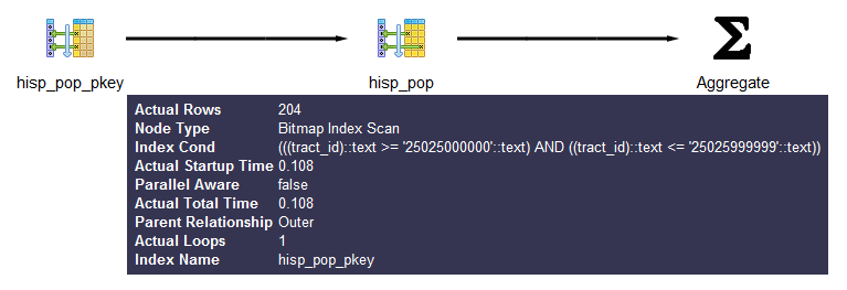
Figure 9-1. Graphical explain output

You can get more detailed information about each part by mousing over the node in the display.

Before wrapping up this section, we must pay homage to the tabular explain plan created by Hubert Lubaczewski. Using his site, you can copy and paste the text output of your EXPLAIN output, and it will show you a beautifully formatted table, as shown in Figure 9-2.

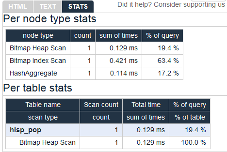
Figure 9-2. Online EXPLAIN statistics

In the HTML tab, you’ll see a nicely reformatted color-coded table of the plan, with problem areas highlighted in vibrant colors, as shown in Figure 9-3. It has columns for exclusive time (time consumed by the parent step) and inclusive time (the time of the parent step plus its child steps).

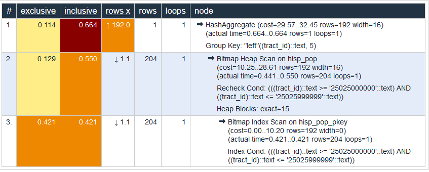
Figure 9-3. Tabular explain output

Although the HTML table in Figure 9-3 provides much the same information as our plain-text output, the color coding and the breakout of numbers makes it easier to digest. For example, yellow, brown, and red highlight potential bottlenecks.

The rows x column is the expected number of rows, while the rows column shows the actual number after execution. This reveals that, although our planner’s final step was expecting 192 records, we ended up with just one. Bad row estimates are often caused by out-of-date table statistics. It’s always a good habit to analyze tables frequently to update the statistics, especially right after an extensive update or insert.

Overusing Subqueries in SELECT

A classic newbie mistake is to think of subqueries as independent entities. Unlike conventional programming languages, SQL doesn’t take kindly to black-boxing—writing a bunch of subqueries independently and then assembling them mindlessly to get the final result. You have to treat each query holistically. How you piece together data from different views and tables is every bit as important as how you go about retrieving the data in the first place.

The unnecessary use of subqueries, as shown in Example 9-7, is a common symptom of piecemeal thinking.

SELECT tract_id,
    (SELECT COUNT(*) FROM census.facts As F 
WHERE F.tract_id = T.tract_id) As num_facts,
    (SELECT COUNT(*)
    FROM census.lu_fact_types As Y
    WHERE Y.fact_type_id IN (
        SELECT fact_type_id
        FROM census.facts F
        WHERE F.tract_id = T.tract_id
    )
    ) As num_fact_types
FROM census.lu_tracts As T;

Example 9-7 can be more efficiently written as Example 9-8. This query, consolidating selects and using a join, is not only shorter than the prior one, but faster. If you have a larger dataset or weaker hardware, the difference could be even more pronounced.

SELECT T.tract_id,
    COUNT(f.fact_type_id) As num_facts,
    COUNT(DISTINCT fact_type_id) As num_fact_types
FROM census.lu_tracts As T LEFT JOIN census.facts As F ON T.tract_id = F.tract_id
GROUP BY T.tract_id;

Figure 9-4 shows the graphical plan for Example 9-7 (we’ll save you the eyesore of seeing the gnarled output of the text EXPLAIN), while Figure 9-5 shows the tabular output from http://explain.depesz.com, revealing a great deal of inefficiency.

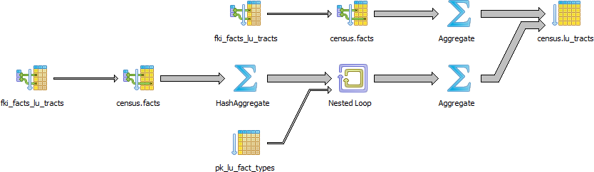
Figure 9-4. Graphical plan when overusing subqueries

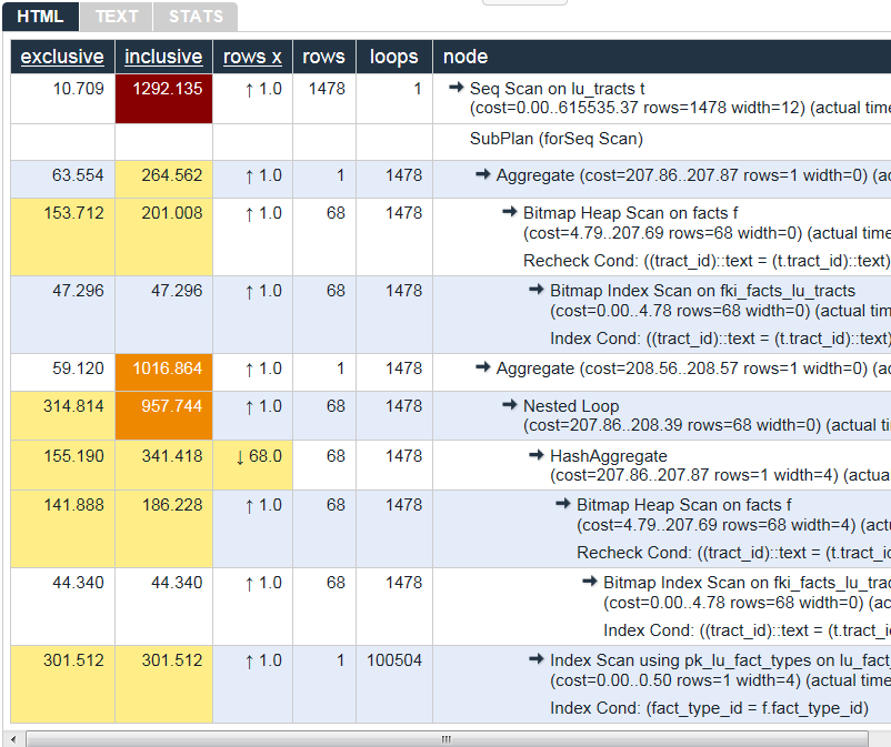
Figure 9-5. Tabular plan when overusing subqueries

Figure 9-6 shows the graphical plan of Example 9-8, demonstrating how much less work goes on in it.

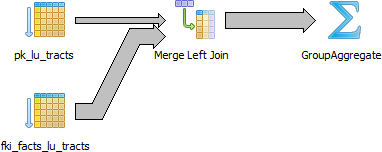
Figure 9-6. Graphical plan after removing subqueries

Keep in mind that we’re not asking you to avoid subqueries entirely. We’re only asking you to use them judiciously. When you do use them, pay extra attention to how you incorporate them into the main query. Finally, remember that a subquery should work with the main query, not independently of it.

Avoid SELECT *

SELECT * is wasteful. It’s akin to printing out a 1,000-page document when you need only 10 pages. Besides the obvious downside of adding to network traffic, there are two other drawbacks that you might not think of.

First, PostgreSQL stores large blob and text objects using TOAST (The Oversized-Attribute Storage Technique). TOAST maintains side tables for PostgreSQL to store this extra data and may chunk a single text field into multiple rows. So retrieving a large field means that TOAST must assemble the data from several rows of a side TOAST table. Imagine the extra processing if your table contains text data the size of War and Peace and you perform an unnecessary SELECT *.

Second, when you define views, you often will include more columns than you’ll need. You might even go so far as to use SELECT * inside a view. This is understandable and perfectly fine. PostgreSQL is smart enough to let you request all the columns you want in your view definition and even include complex calculations or joins without incurring penalty, as long as no user runs a query referring to individual columns.

To drive home our point, let’s wrap our census in a view and use the slow subquery example from Example 9-7:

CREATE OR REPLACE VIEW vw_stats AS
SELECT tract_id,
    (SELECT COUNT(*) 
      FROM census.facts As F 
      WHERE F.tract_id = T.tract_id) As num_facts,
    (SELECT COUNT(*)
      FROM census.lu_fact_types As Y
      WHERE Y.fact_type_id IN (
        SELECT fact_type_id
        FROM census.facts F
        WHERE F.tract_id = T.tract_id
    )
    ) As num_fact_types
FROM census.lu_tracts As T;

Now we query our view with this query:

SELECT tract_id FROM vw_stats;

Execution time is about 21 ms on our server because it doesn’t run any computation for certain fields such as num_facts and num_fact_types, fields we did not ask for. If you looked at the plan, you may be startled to find that it never even touches the facts table because it’s smart enough to know it doesn’t need to. But suppose we enter:

SELECT * FROM vw_stats;

Our execution time skyrockets to 681 ms, and the plan is just as we had in Figure 9-4. Although our results in this example suffer the loss of just milliseconds, imagine tables with tens of millions of rows and hundreds of columns. Those milliseconds could translate into overtime at the office waiting for a query to finish.

Make Good Use of CASE

We’re always surprised how frequently people forget about using the ANSI SQL CASE expression. In many aggregate situations, a CASE can obviate the need for inefficient subqueries. We’ll demonstrate the point with two equivalent queries and their corresponding plans. Example 9-9 uses subqueries.

SELECT T.tract_id, COUNT(*) As tot, type_1.tot AS type_1
FROM
    census.lu_tracts AS T LEFT JOIN
    (SELECT tract_id, COUNT(*) As tot
        FROM census.facts
        WHERE fact_type_id = 131
        GROUP BY tract_id
    ) As type_1 ON T.tract_id = type_1.tract_id LEFT JOIN
    census.facts AS F ON T.tract_id = F.tract_id
GROUP BY T.tract_id, type_1.tot;

Figure 9-7 shows the graphical plan of Example 9-9.

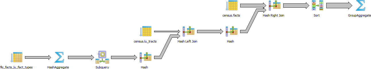
Figure 9-7. Graphical plan when using subqueries instead of CASE

We now rewrite the query using CASE. You’ll find that the economized query, shown in Example 9-10, is generally faster and much easier to read.

SELECT T.tract_id, COUNT(*) As tot,
    COUNT(CASE WHEN F.fact_type_id = 131 THEN 1 ELSE NULL END) AS type_1
FROM census.lu_tracts AS T LEFT JOIN census.facts AS F
ON T.tract_id = F.tract_id
GROUP BY T.tract_id;

Figure 9-8 shows the graphical plan of Example 9-10.

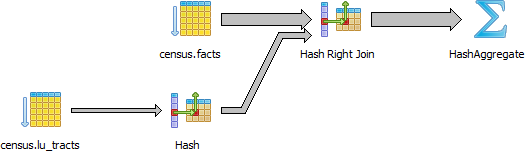
Figure 9-8. Graphical explain when using CASE

Even though our rewritten query still doesn’t use the fact_type index, it’s faster than using subqueries because the planner scans the facts table only once. A shorter plan is generally not only easier to comprehend but also often performs better than a longer one, although not always.

Using FILTER Instead of CASE

PostgreSQL 9.4 introduced the FILTER construct, which we introduced in “FILTER Clause for Aggregates”. FILTER can often replace CASE in aggregate expressions. Not only is this syntax more pleasant to look at, but in many situations it performs better. We repeat Example 9-10 with the equivalent filter version in Example 9-11.

SELECT T.tract_id, COUNT(*) As tot,
    COUNT(*) FILTER (WHERE F.fact_type_id = 131) AS type_1
FROM census.lu_tracts AS T LEFT JOIN census.facts AS F
ON T.tract_id = F.tract_id
GROUP BY T.tract_id;

For this particular example, the FILTER performance is only about a millisecond faster than our CASE version, and the plans are more or less the same.

What Does a Parallel Query Plan Look Like?

How do you know if your query is a beneficiary of parallelization? Look in the plan. Parallelization is done by a part of the planner called a gather node. So if you see a gather node in your query plan, you have some kind of parallelization. A gather node contains exactly one plan, which it divides amongst what are called workers. Each worker runs as separate backend processes, each process working on a portion of the overall query. The results of workers are collected by a worker acting as the leader. The leader does the same work as other workers but has the added responsibility of collecting all the answers from fellow workers. If the gather node is the root node of a plan, the whole query will be run in parallel. If it’s lower down, only the subplan it encompasses will be parallelized.

For debugging purposes, you can invoke a setting called force_parallel_mode. When true, it will encourage the planner to use parallel mode if a query is parallelizable even when the planner concludes it’s not cost-effective to do so. This setting is useful during debugging to figure out why a query is not parallelized. Don’t switch on this setting in a production environment, though!

The queries you’ve seen thus far in this chapter will not trigger a parallel plan because the cost of setting up the background workers outweighs the benefit. To confirm that our query takes longer when forced to be parallel, try the following:

set force_parallel_mode = true;

And then run Example 9-4 again. The output of the new plan is shown in Example 9-12.

Gather
    (cost=1029.57..1051.65 rows=192 width=64)
    (actual time=12.881..13.947 rows=1 loops=1)
    Workers Planned: 1
    Workers Launched: 1
    Single Copy: true
    -> HashAggregate
        (cost=29.57..32.45 rows=192 width=64)
        (actual time=0.230..0.231 rows=1 loops=1)
        Group Key: "left"((tract_id)::text, 5)
        -> Bitmap Heap Scan on hisp_pop
            (cost=10.25..28.61 rows=192 width=36)
            (actual time=0.127..0.184 rows=204 loops=1)
            Recheck Cond:
                (((tract_id)::text >= '25025000000'::text) AND
                ((tract_id)::text <= '25025999999'::text))
                -> Bitmap Index Scan on hisp_pop_pkey
                    (cost=0.00..10.20 rows=192 width=0)
                    (actual time=0.106..0.106 rows=204 loops=1)
                    Index Cond:
                        (((tract_id)::text >= '25025000000'::text) AND
                        ((tract_id)::text <= '25025999999'::text))
Planning time: 0.416 ms
Execution time: 16.160 ms

The cost of organizing additional workers (even one) significantly increases the total time of the query.

Generally, parallelization is rarely worthwhile for queries that finish in a few milliseconds. But for queries over a ginormous dataset that normally take seconds or minutes to complete, parallelization is worth the initial setup cost.

To illustrate the benefit of parallelization, we downloaded a table from the US Bureau of Labor Statistics with 6.5 million rows of data and ran the query in Example 9-13.

set max_parallel_workers_per_gather=4;
EXPLAIN ANALYZE VERBOSE
SELECT COUNT(*), area_type_code
FROM labor
GROUP BY area_type_code
ORDER BY area_type_code;

Finalize GroupAggregate
    (cost=104596.49..104596.61 rows=3 width=10)
    (actual time=500.440..500.444 rows=3 loops=1)
    Output: COUNT(*), area_type_code
    Group Key: labor.area_type_code
    -> Sort
        (cost=104596.49..104596.52 rows=12 width=10)
        (actual time=500.433..500.435 rows=15 loops=1)
        Output: area_type_code, (PARTIAL COUNT(*))
        Sort Key: labor.area_type_code
        Sort Method: quicksort  Memory: 25kB
        -> Gather
            (cost=104595.05..104596.28 rows=12 width=10)
            (actual time=500.159..500.382 rows=15 loops=1)
            Output: area_type_code, (PARTIAL COUNT(*))
            Workers Planned: 4
            Workers Launched: 4
            -> Partial HashAggregate
                (cost=103595.05..103595.08 rows=3 width=10)
                (actual time=483.081..483.082 rows=3 loops=5)
                Output: area_type_code, PARTIAL count(*)
                Group Key: labor.area_type_code
                Worker 0: actual time=476.705..476.706 rows=3 loops=1
                Worker 1: actual time=480.704..480.705 rows=3 loops=1
                Worker 2: actual time=480.598..480.599 rows=3 loops=1
                Worker 3: actual time=478.000..478.000 rows=3 loops=1
                -> Parallel Seq Scan on public.labor
                    (cost=0.00..95516.70 rows=1615670 width=2)
                    (actual time=1.550..282.833 rows=1292543 loops=5)
                    Output: area_type_code
                    Worker 0: actual time=0.078..282.698 rows=1278313 loops=1
                    Worker 1: actual time=3.497..282.068 rows=1338095 loops=1
                    Worker 2: actual time=3.378..281.273 rows=1232359 loops=1
                    Worker 3: actual time=0.761..278.013 rows=1318569 loops=1
Planning time: 0.060 ms
Execution time: 512.667 ms

To see the cost and timing without parallelization, set max_parallel_workers_per_gather=0, and compare the plan, as shown in Example 9-14.

set max_parallel_workers_per_gather=0;
EXPLAIN ANALYZE VERBOSE
SELECT COUNT(*), area_type_code
FROM labor
GROUP BY area_type_code
ORDER BY area_type_code;

Sort
    (cost=176300.24..176300.25 rows=3 width=10)
    (actual time=1647.060..1647.060 rows=3 loops=1)
    Output: (COUNT(*)), area_type_code
    Sort Key: labor.area_type_code
    Sort Method: quicksort  Memory: 25kB
    -> HashAggregate
        (cost=176300.19..176300.22 rows=3 width=10)
        (actual time=1647.025..1647.025 rows=3 loops=1)
        Output: count(*), area_type_code
        Group Key: labor.area_type_code
        -> Seq Scan on public.labor
            (cost=0.00..143986.79 rows=6462679 width=2)
            (actual time=0.076..620.563 rows=6462713 loops=1)
            Output: series_id, year, period, value, footnote_codes, area_type_code
Planning time: 0.054 ms
Execution time: 1647.115 ms

In both cases, the output is the following:

count   | area_type_code
--------+---------------
3718937 | M
2105205 | N
 638571 | S
(3 rows)

In the parallel plan, four workers each take about 280 ms to accomplish their portion of the task.

Parallel Scans

A parallel query has a particular scan strategy for partitioning the set of data among workers. In PostgreSQL 9.6, only a sequential scan is parallelizable. PostgreSQL 10 is also able to parallelize bitmap heap scans, index scans, and index-only scans. However, for index and index-only scans, only B-Tree indexes will parallelize. No such limitation exists for bitmap heap scans: for them, any index type will qualify. But in the bitmap heap scan, the building of the bitmap index is not parallelizable, so workers must wait for the bitmap index to be fully built.

Parallel Joins

Joins also benefit from parallelization. In PostgreSQL 9.6, nested loops and hash joins are parallelizable.

In nested loops, each worker matches its subset of data against a complete reference set of data shared by all workers.

In hash joins, each worker builds a separate copy of the hash table and joins this with their partitioned share of other tables. Thus, in a hash join, workers are doing redundant work by doing a full hash. So in cases where creating the hash table is expensive, a parallel hash join is less efficient than a nonparallel join.

In PostgreSQL 10, merge joins are parallelizable. Merge joins have a similar limitation to hash joins, in that one side of the join is repeated in its entirety by each worker.

Strategy Settings

Although the PostgreSQL query planner doesn’t accept index hints as some other database products do, you can disable various strategy settings on a per-query or permanent basis to dissuade the planner from going down an unproductive path. All planner optimizing settings are documented in the section Planner Method Configuration of the manual. By default, all strategy settings are enabled, arming the planner with maximum flexibility. You can disable various strategies if you have some prior knowledge of the data. Keep in mind that disabling doesn’t necessarily mean that the planner will be barred from using the strategy. You’re only making a polite request to the planner to avoid it.

Two settings that we occasionally disable are enable_nestloop and enable_seqscan. The reason is that these two strategies tend to be the slowest, though not in all cases. Although you can disable them, the planner can still use them when it has no viable alternative. When you do see them being used, it’s a good idea to double-check that the planner is using them out of efficiency, and not out of ignorance. One quick way to check is to disable them. If they are used by default but not used when you disable them, compare the actual costs between the two cases to confirm that using them is more efficient than not using them.

How Useful Is Your Index?

When the planner decides to perform a sequential scan, it loops through all the rows of a table. It opts for this route when it finds no index that could satisfy a query condition, or it concludes that using an index is more costly than scanning the table. If you disable the sequential scan strategy, and the planner still insists on using it, this means that indexes are missing or that the planner can’t use the indexes you have in place for the particular query. Two common mistakes people make are to leave useful indexes out of their tables or to put in indexes that can’t be used by their queries. An easy way to check whether your indexes are being used is to query the pg_stat_user_indexes and pg_stat_user_tables views. To target slow queries, use the pg_stat_statements extension described in “Gathering Statistics on Statements”.

Let’s start off with a query against the table we created in Example 7-22. We’ll add a GIN index on the array column. GIN indexes are among the few indexes you can use to index arrays:

CREATE INDEX idx_lu_fact_types ON census.lu_fact_types USING gin (fact_subcats);

To test our index, we’ll execute a query to find all rows with subcats containing “White alone” or “Asian alone.” We explicitly enabled sequential scan even though it’s the default setting, just to be sure. The accompanying EXPLAIN output is shown in Example 9-15.

set enable_seqscan = true;
EXPLAIN (ANALYZE)
SELECT *
FROM census.lu_fact_types
WHERE fact_subcats && '{White alone, Black alone}'::varchar[];

Seq Scan on lu_fact_types
    (cost=0.00..2.85 rows=2 width=200)
    actual time=0.066..0.076 rows=2 loops=1)
	Filter: (fact_subcats 
&& '{"White alone","Black alone"}'::character varying[])
	Rows Removed by Filter: 66
Planning time: 0.182 ms
Execution time: 0.108 ms

Observe that when enable_seqscan is enabled, our index is not being used and the planner has chosen to do a sequential scan. This could be because our table is so small or because the index we have is no good for this query. If we repeat the query but turn off sequential scan beforehand, as shown in Example 9-16, we can see that we have succeeded in forcing the planner to use the index.

set enable_seqscan = false;
EXPLAIN (ANALYZE)
SELECT *
FROM census.lu_fact_types
WHERE fact_subcats && '{White alone, Black alone}'::varchar[];

Bitmap Heap Scan on lu_fact_types
	(cost=12.02..14.04 rows=2 width=200)
    (actual time=0.058..0.058 rows=2 loops=1)
	Recheck Cond: (fact_subcats 
&& '{"White alone","Black alone"}'::character varying[])
	Heap Blocks: exact=1
		-> Bitmap Index Scan on idx_lu_fact_types
        (cost=0.00..12.02 rows=2 width=0)
        (actual time=0.048..0.048 rows=2 loops=1)
        Index Cond: (fact_subcats 
&& '{"White alone","Black alone"}'::character varying[])
Planning time: 0.230 ms
Execution time: 0.119 ms

From this plan, we learn that our index can be used but ends up making the query take longer because the cost is more than doing a sequential scan. Therefore, under normal circumstances, the planner will opt for the sequential scan. As we add more data to our table, we’ll probably find that the planner changes strategies to an index scan.

In contrast to the previous example, suppose we were to write a query of the form:

SELECT * FROM census.lu_fact_types WHERE 'White alone' = ANY(fact_subcats);

We would discover that, regardless of how we set enable_seqscan, the planner will always perform a sequential scan because the index we have in place can’t service this query. So it is important to consider which indexes will be useful and to write queries to take advantage of them. And experiment, experiment, experiment!

Table Statistics

Despite what you might think or hope, the query planner is not a magician. Its decisions follow prescribed logic that’s far beyond the scope of this book. The rules that the planner follows depend heavily on the current state of the data. The planner can’t possibly scan all the tables and rows prior to formulating its plan. That would be self-defeating. Instead, it relies on aggregated statistics about the data.

Therefore, having accurate and current stats is crucial for the planner to make the right decision. If stats differ greatly from reality, the planner will often come up with bad plans, the most detrimental of these being unnecessary sequential table scans. Generally, only about 20 percent of the entire table is sampled to produce stats. This percentage could be even lower for very large tables. You can control the number of rows sampled on a column-by-column basis by setting the STATISTICS value.

To get a sense of the information culled and used by the planner, query the pg_stats table, as illustrated in Example 9-17.

SELECT
    attname As colname,
    n_distinct,
    most_common_vals AS common_vals,
    most_common_freqs As dist_freq
FROM pg_stats
WHERE tablename = 'facts'
ORDER BY schemaname, tablename, attname;

colname      | n_distinct | common_vals      | dist_freq
-------------+------------+------------------+------------------------------
fact_type_id |         68 | {135,113...      | {0.0157,0.0156333,...
perc         |        985 | {0.00,...        | {0.1845,0.0579333,0.056...
tract_id     |       1478 | {25025090300...  | {0.00116667,0.00106667,0.0...
val          |       3391 | {0.000,1.000,2...| {0.2116,0.0681333,0...
yr           |          2 | {2011,2010}      | {0.748933,0.251067}

pg_stats gives the planner a sense of how actual values are dispersed within a given column and lets it plan accordingly. The pg_stats table is constantly updated as a background process. After a large data load or a major deletion, you should manually update the stats by executing VACUUM ANALYZE. VACUUM permanently removes deleted rows from tables; ANALYZE updates the stats.

For columns that participate often in joins and are used heavily in WHERE clauses, consider increasing the number of sampled rows:

ALTER TABLE census.facts ALTER COLUMN fact_type_id SET STATISTICS 1000;

Version 10 introduced support for multicolumn stats via the new CREATE STATISTICS DDL construct. This feature allows you to create stats against a combination of columns. A multicolumn stat is useful if you have columns that are correlated in value. Say, for example, that you have a particular kind of data for only one year and not other years. In that case, you might want to create a compound stat for fact_type_id and yr as shown in Example 9-18.

CREATE STATISTICS census.stats_facts_type_yr_dep_dist (dependencies, ndistinct)
                ON fact_type_id, yr FROM census.facts;
ANALYZE census.facts;

A CREATE STATISTICS statement must specify two or more columns in a single table. Example 9-18 creates stats on the columns fact_type_id and yr in the census.facts table. The statistics should also be named, although that is optional. If you specify a schema as part of the name, the statistics will be created in that schema; otherwise, they get created in the default schema.

You can collect two kinds of statistics, and must specify one or both in your statement:

• The dependencies statistic catalogs dependencies between columns. For example, zip code 02109 is seen only with Boston in the city column. dependencies statistics are used only to optimize queries with equalities, such as a query specifying city = 'Boston' and zip = '02109'.

• The ndistinct statistic catalogs how often column values are seen together and tries to catalog statistics for each group of columns. ndistinct statistics are only used for improving GROUP BY clauses. Specifically, they are useful only on queries that group by all the columns in your statistic.

Statistics created using CREATE STATISTICS are stored in the table pg_statistic_ext and can be dropped using DROP STATISTICS. Similar to other statistics, they are computed during an ANALYZE run, which happens during the system vacuum analyze process. After creating a table, it’s a good idea to run an ANALYZE on it so the new stats can be used immediately.

Random Page Cost and Quality of Drives

Another setting that influences the planner is the random_page_cost (RPC) ratio, which is the relative cost of disk access when retrieving a record using a sequential read versus random access. Generally, the faster (and more expensive) the physical disk, the lower the ratio. The default value for RPC is 4, which works well for most mechanical hard drives on the market today. The use of solid-state drives (SSDs), high-end storage area networks (SANs), or cloud storage makes it worth tweaking this value.

You can set the RPC ratio per database, per server, or per tablespace. At the server level, it makes most sense to set the ratio in the postgresql.conf file. If you have different kinds of disks, you can set the values at the tablespace level using the ALTER TABLESPACE command:

ALTER TABLESPACE pg_default SET (random_page_cost=2);

Details about this setting can be found at Random Page Cost Revisited. The article suggests the following settings:

• High-end NAS/SAN: 2.5 or 3.0

• Amazon EBS and Heroku: 2.0

• iSCSI and other mediocre SANs: 6.0, but varies widely

• SSDs: 2.0 to 2.5

• NvRAM (or NAND): 1.5