Due to the nature of microservice architecture, you may end up with many services to meet product needs. Having good visibility of this system becomes important for being proactive about spotting problems and taking quick action to fix them. Services talk to other services, databases, queues, and third-party services, which produces insights about internal operations. In this chapter, we learn how to collect those insights and generate meaningful reports to understand situations in a cloud-native microservices environment.
Microservice architecture is a distributed system in which services communicate to maintain data consistency. Let’s say that PlaceOrder visits three services to create an order, charge a customer’s credit card, and ship it to the customer. An error can occur in any of those services while handling a PlaceOrder operation, and this is where the challenge begins. Observability helps us track a problem’s root cause by analyzing traces, metrics, and logs. This chapter will show how observability can be perfectly handled in a microservices system that uses gRPC for communication. In this context, observability can answer the following questions:
Why is performance degraded in the middle of the day each Thursday?
What is the performance of the Payment service like right now?
To answer these questions, we need a proper observability system that shows traces, metrics, and logs in the correct format so that we can analyze them and take action. We will use different technologies such as Jaeger (https://www.jaegertracing.io/), OpenTelemetry (https://opentelemetry.io/), and Prometheus (https://prometheus.io/), but first let’s look at what traces, metrics, and logs are in a microservices environment.
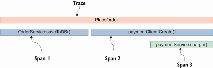
A trace, a collection of operations to handle a unique transaction, refers to the journey of a request across services in a distributed system. It encodes the metadata of a specific request to propagate it until it reaches its final service. A trace can contain one or more spans that map to a single operation (see figure 9.1).
As shown in figure 9.1, the name of the journey is PlaceOrder, and once it is initialized, a trace ID is automatically generated. Then it spans to multiple parts such as saving in the database and then calling the Payment service via the payment client. The payment client call process also creates another span while it is in the Payment service to make a query in a logging backend using a trace ID and sorting it by date in ascending order to see what happened to the request. We can see gRPC-related metadata in spans under a specific trace (figure 9.2).
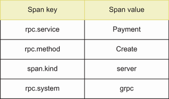
Figure 9.2 is for a sever span that contains information about a single operation: the entry point of payment.Create. Keys are already implemented within the specific instrumentation library contracted by the OpenTelemetry project. (You can see all instrumentation libraries here https://opentelemetry.io/docs/instrumentation/.) rpc .service and rpc.method refer to the gRPC service name and gRPC method name under that service, respectively. span.kind is used for pointing out if instrumentation is done on either the client or server side. Finally, rpc.system shows what sort of RPC is used in service communication, in this case gRPC. Now that we understand how trace and span work together, let’s look at what metrics we can have in a microservices environment.
Metrics contain numerical values to help us define a service’s behavior over time. Prometheus has metrics that are defined by name, value, label, and timestamp. Using these fields, we can see metrics over time. We can also group them using their labels. Of course, we can apply other aggregation techniques (https://prometheus.io/docs/prometheus/latest/querying/functions/) using metric fields, SLA, SLO, and SLI, and obtain information about the system. For more in-depth information, see Google’s Site Reliability Engineering book (https://sre.google/sre-book/table-of-contents/).
An SLA (service-level agreement) is an agreement between customers and service providers and contains measurable metrics such as latency, throughput, and uptime. It is not easy to measure and report SLAs, so a stable observability system is important.
An SLI (service-level indicator) is a specific metric that helps showcase service quality to customers by referencing request latency, error rate, and throughput for example. The statement “The throughput of our service is 1000/ms” indicates that this service can handle 1,000 operations per millisecond.
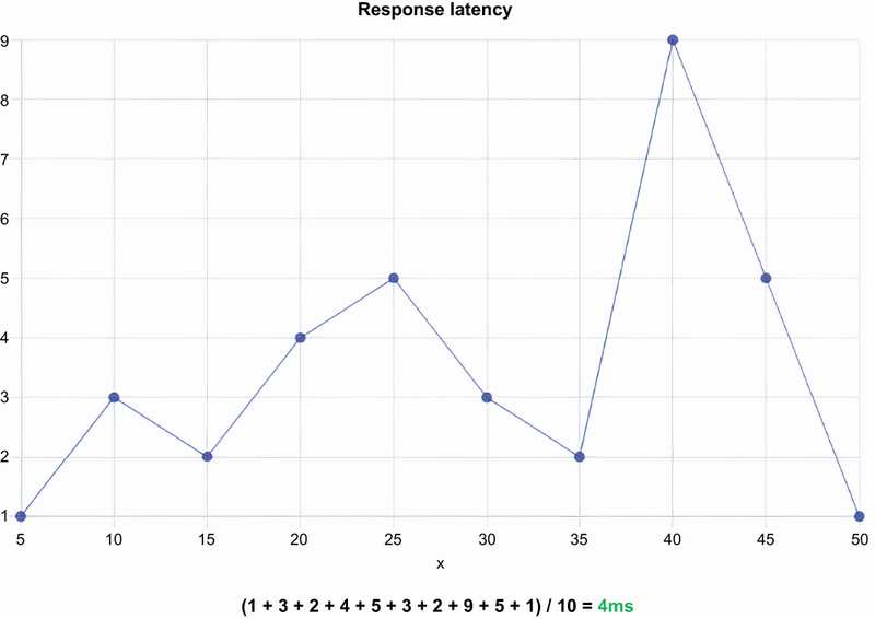
A SLO (service-level objective) is the goal for a product team to satisfy SLA. Especially in SaaS projects, you can see the SLA in terms and conditions pages. A typical example of a SLO is “99.999% uptime for the Object Storage service”: the Object Storage service should be up 99.999%, and it might be down 0.001% of the time. These numbers are calculated as average values (figure 9.3).
As you can see in figure 9.3, the result is found by adding latency amounts (ms) and dividing them by the sampling count of 10. This is also called the average value of numbers. If I was using SLA documentation, I would say, “We provide a 4 ms response latency guarantee for our services.” Can you spot the problem here? What if you have a 1,000 times 1 ms response latency and ten times 4 seconds latency?
10,00 x 1 ms + 10 x 4,000 ms = 5,000 ms
Even though you had a very good response latency of 1 ms, the remaining ten response latencies corrupted your report. Averaging numbers may not satisfy customers; they might want to see the distribution of latencies with their percentages. There is a term to explain this situation: percentile. For example, if you say, “The 95th percentile response latency is 3 ms,” 95% of the response latencies are 3 ms or less.
Think about the response latency numbers in figure 9.4.
The first thing we can do is sort all the numbers in descending order, which results in the numbers shown in figure 9.5.
To find 80th percentile response latency, see the index at 80% from the right to left direction, which in this case is 11 ms.
Applications produce events, and it is important to be aware of them to take action in case of an error or any kind of warning message. In this section, we will check the logging architecture first, then set up a logging system to ship gRPC microservices logs to the logging backend.
In monolithic applications, saving produced logs in a file to read later is not difficult. In microservices, you can still save logs in files, but combining different log files is challenging. Saving logs locally is not the only option; we can also ship them to a central location. In a Kubernetes environment, we have two types of logging architecture:
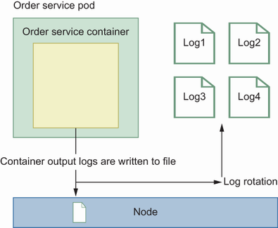
In node-level logging architecture, applications generate events, which are logged to a file or standard output using some logging library in the application. If the application keeps logging events, that file can grow dramatically, which will make it hard to find certain logs. To avoid this situation, we can use log rotation: once a log file reaches a specific size, it can be rotated to a file with a name that contains time metadata for that rotation. Once you rotate logs, they are saved in separate files, but we still need to ship them to a central location or find a way to analyze them in multiple files (figure 9.6).
Some libraries can collect all the logs from containers and generate other artifacts.
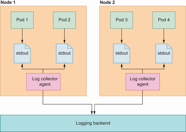
There are agents, typically a daemonset, on each Kubernetes cluster node that are responsible for collecting logs from container-standard output logs. In cluster-level logging architecture, the logs are saved to a file on the host, but this time a central agent, (e.g., Elasticsearch, https://www.elastic.co/; graylog, https://www.graylog.org/) collects those logs and sends them to the logging backend. In figure 9.7, logging backends are not simply services that accept logging requests and serve them; they can also have components to show dashboards about logs and create alarms.
You have probably heard about the ELK stack, Elasticsearch-Logstash-Kibana: Elasticsearch is the logging backend, Logstash is some kind of log collector, and Kibana is the UI for logs, a proper monitoring dashboard for gRPC microservices that gives insight into services such as error rates and check details. We can even create alarms to send a notification to the development team if there is a matching log pattern in the logging backend store. Now that we understand tracing, metrics, and logs, let’s look at how these work in the Kubernetes environment.
OpenTelemetry (https://opentelemetry.io/) is a collection of SDKs and APIs that helps applications generate, collect, and export metrics, traces, and log information. OpenTelemetry is an umbrella project; you can see the implementation in different languages. We will use this project’s Go version (https://opentelemetry.io/docs/instrumentation/go/). How can OpenTelemetry help us in a gRPC microservices project? Let’s see the answer together.
In a gRPC microservices project, services contact each other, so the client connection is a good candidate for generating insight into an application. When a client connects to the server, we can also generate observability data on the server side. We can even collect insights from database-related calls, and we already have an OpenTelemetry GORM extension (https://github.com/uptrace/opentelemetry-go-extra/tree/main/otelgorm) that helps us collect DB operations. With proper instrumentation setup, we can also allow OpenTelemetry plug-ins to propagate tracing information to the next services. Let’s look at how to handle collection with minimum effort.
In the gRPC world, it is very common to use interceptors to handle common things in a central place instead of implementing them manually by duplicating different packages. Instrumentation has gRPC support—a set of interceptors that collect gRPC metrics and make them available to send to metric collector backend such as Jaeger. Once we add these interceptors to client calls, the Order service calls the Payment service via the payment adapter, and all the requests to the Payment service are intercepted to collect data and make it available to ship to the metric backend:
...
var opts []grpc.DialOption
    opts = append(opts,
        grpc.WithTransportCredentials(insecure.NewCredentials()),
        grpc.WithUnaryInterceptor(otelgrpc.UnaryClientInterceptor()),   ❶
    )
    conn, err := grpc.Dial(paymentServiceUrl, opts...)
...
❶ An interceptor for OpenTelemetry gRPC integration
In chapter 5, we used gRPC interceptors to handle retry operations and create resilient systems. In this example, we use the same notation by adding an interceptor to a dial option so that the client connection will know how to collect and send telemetry data. In our case, telemetry data is generated while the Order service calls the Payment service.
The next step is to add those instrumentations to our codebase and first look at how we can prepare a metric backend, then provide the metrics’ backend URL for instrumentation.
gRPC microservices generate metrics for different components, and those metrics become helpful if we process them to generate actionable reports. OpenTelemetry SDKs help us instrument gRPC microservices quickly and require a metric collector endpoint to send them for future processing. We will use Jaeger, an open source distributed tracing system developed by Uber Technologies, to store our metrics and generate meaningful dashboards to understand what is happening in the microservices environment. Jaeger is good for handling metrics that come from OpenTelemetry; it uses a metric store such as Cassandra to complete a set of queries to show it in the Jaeger UI. Jaeger also allows us to save metrics in another store such as Prometheus to show microservices’ performance in a monitoring dashboard.
Next, we will complete a step-by-step installation of observability tools to collect and visualize system insights. Let’s look at the overall picture metrics’ backend architecture; then we can continue with Kubernetes-related operations.
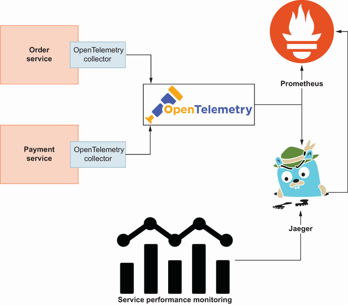
In the service performance monitoring component of Jaeger (figure 9.8), applications send OpenTelemetry data to the Jaeger collector endpoint, and Jaeger also sends it to Prometheus to store it in a time series format. Since we have time series data, it is easy for Jaeger to generate response latency graphs based on time using Prometheus queries. This will show percentile metrics over time.
In the Jaeger UI, we also see a tracing query screen to find traces by service name and check request flow by their latencies. For example, we can see the latency distribution for each service after the client sends a PlaceOrder request. Now that we understand the initial picture of the metrics backend and what we can do with Jaeger components, let’s go back to the Kubernetes environment and set up all those architectures for observability.
As mentioned, we will use Jaeger and Prometheus for our metrics backend. To install them, we will use Helm Chart, a dependency management tool for the Kubernetes environment. Plenty of charts help install Jaeger, but because there is no option with both Prometheus and Jaeger, I implemented one (https://artifacthub.io/packages/helm/huseyinbabal/jaeger) that includes three components: Jaeger All in One, which has all Jaeger components; OpenTelemetry Collector for collector endpoint; and Prometheus. Let’s look at what kind of information they expose.
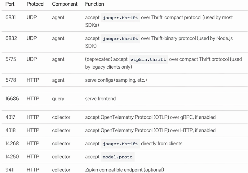
Jaeger All in One uses the jaegertracing/all-in-one (https://hub.docker.com/r/jaegertracing/all-in-one/) Docker image to serve Jaeger components. We will use Helm Chart to deploy this, which exposes the ports in figure 9.9 (http://mng.bz/KeGE).
These ports are primarily used in Jaeger-related operations, such as viewing metrics on the Jaeger UI. gRPC microservices will also send their traces to the OpenTelemetry Collector in the Helm Chart. Let’s look at what the OpenTelemetry Collector exposes for gRPC microservices.
OpenTelemetry Collector uses otel/opentelemetry-collector-contrib (https://hub.docker.com/r/otel/opentelemetry-collector-contrib), which exposes two ports: 14278 and 8889. 14278 is for the collector endpoint; it accepts metric requests from gRPC microservices. 8889 is used for the Prometheus exporter, and Jaeger uses this port to get time series data for performance monitoring. Once the collector obtains the values, it also sends calculated data to Prometheus.
We need Prometheus for Jaeger to store service insights in a time series format. The Helm Chart also provisions Prometheus, but you may want the existing Prometheus to be used in Jaeger All in One deployment. We can add the following environment variables to the Jaeger All in One deployment to enable the Prometheus metrics storage type:
METRICS_STORAGE_TYPE=prometheus
PROMETHEUS_SERVER_URL=http://jaeger-
➥ prometheus.jaeger.svc.cluster.local:9090
jaeger-prometheus is the Prometheus service name, jaeger is the namespace, and svc.cluster.local is the suffix used for Kubernetes service discovery. Now that we know all the components in the Helm Chart, let’s deploy them to our local Kubernetes cluster.
We must add a repo for the Helm Chart with the following command:
helm repo add huseyinbabal https://huseyinbabal.github.io/charts
It will add my repo to your local Helm repositories list. Then we are ready to deploy Jaeger with all components:
helm install my-jaeger huseyinbabal/jaeger -n jaeger –create-namespace
This will install all the resources in the jaeger namespace, which will be created if it does not already exist. You can verify the installation by checking if Jaeger, OpenTelemetry, and Prometheus pods exist in your cluster.
Now that we have our metrics backend ready, we can continue changing our microservices to use OpenTelemetry SDKs to send data to the collector endpoint (http://jaeger-otel.jaeger.svc.cluster.local:14278/api/traces). Traces are sent to the OpenTelemetry Collector.
In this section, we will add the OpenTelemetry interceptor to the Order service, which will collect server-side metrics. Regardless of who calls the Order service, traces and metrics will be sent to the Jaeger OpenTelemetry Collector URL. To enable such a feature in the gRPC service, we will do two things:
When you configure a tracing provider, you enable a global tracing configuration in your project, and that is the entry point of our services: main.go. This configuration includes adding an exporter, the Jaeger exporter in our case, and configuring the metadata so that tracing SDK can expose that metadata to the tracing collector. This collection operation is handled in batches, meaning the server-side metrics will be collected and sent in a batch instead of sending each metric individually. Here’s the high-level implementation of this provider config:
import (
    "go.opentelemetry.io/otel"
    "go.opentelemetry.io/otel/attribute"
    "go.opentelemetry.io/otel/exporters/jaeger"
    "go.opentelemetry.io/otel/sdk/resource"
    tracesdk "go.opentelemetry.io/otel/sdk/trace"
    semconv "go.opentelemetry.io/otel/semconv/v1.10.0"
)
...
func tracerProvider(url string) (*tracesdk.TracerProvider, error) {
    exp, err := jaeger.New(jaeger.WithCollectorEndpoint(jaeger.WithEndpoint(url)))   ❶
    if err != nil {
        return nil, err
    }
    tp := tracesdk.NewTracerProvider(
        tracesdk.WithBatcher(exp),                                                   ❷
        tracesdk.WithResource(resource.NewWithAttributes(
            semconv.SchemaURL,                                                       ❸
            semconv.ServiceNameKey.String(service),                                  ❹
            attribute.String("environment", environment),
            attribute.Int64("ID", id),                                               ❺
        )),
    )
    return tp, nil
}
❶ Configures the Jaeger exporter
❷ Exports the tracing metrics in a batch
❸ The URL that contains the OpenTelemetry schema
❹ An attribute that describes the service name
❺ An arbitrary ID that can be used in tracing the dashboard
This tracing configuration define service metadata that will be used globally. You can see metadata attributes such as service name, ID, and environment added to the tracing provider configuration. We can see those attributes in the Jaeger tracing UI and search by those attributes. SchemaURL also understands the schema contract of telemetry data.
To use this function in the Order Service, go to the order folder in the microservices project and add the function to the cmd/main.go file. You can automatically execute go mod tidy to fetch the newly added function dependencies. As you can see, this is only a function definition; to initialize the tracing provider, we can add it to the beginning of the main function:
func main() {
    tp, err := tracerProvider("http://jaeger-
    ➥ otel.jaeger.svc.cluster.local:14278/api/traces")   ❶
    if err != nil {
        log.Fatal(err)
    }

    otel.SetTracerProvider(tp)                            ❷
    otel.SetTextMapPropagator(propagation.NewCompositeTextMapPropagator(pro
    ➥ pagation.TraceContext{}))                          ❸
    ...
}
❷ Sets the tracing provider through the OpenTelemtry SDK
❸ Configures the propagation strategy
In the tracing provider configuration, we simply provide a tracing collect endpoint, which we installed via the Helm Chart, and set the tracing provider using OpenTelemetry SDK. Then we configure the propagation strategy to propagate traces and spans from one service to another. For example, since the Order service calls the Payment service to charge a customer, existing trace metadata will be propagated to the Payment service to see the whole request flow in the Jaeger tracing UI. Now that the Order service knows the tracing provider, let’s add a tracing interceptor to the gRPC service.
OpenTelemetry has a registry system in which you can see various instrumentation libraries (https://opentelemetry.io/registry/). When you search for gRPC, you can find gRPC instrumentation that contains a gRPC interceptor. We can add our interceptor as an argument to the gRPC server in this file. Remember that we already have a gRPC server implementation in each service, which you can see in internal/adapters/ grpc/server.go:
import (
"go.opentelemetry.io/contrib/instrumentation/google.golang.org/grpc/otelgrpc"
)
...
grpcServer := grpc.NewServer(
        grpc.UnaryInterceptor(otelgrpc.UnaryServerInterceptor()),
    )
...
Notice that interceptor comes from the otelgrpc package, which you can find in the OpenTelemetry instrumentation registry. Now, whenever we call the Order service, the server metrics will be sent to the Jaeger OpenTelemetry Collector endpoint and be accessible from the Jaeger UI. You can find the pod named jaeger and do a port forward for port 16686, Jaeger’s UI port. For example, if the pod name is jaeger-c55bf4988-ghfsd, the following command in the terminal will open a proxy for port 16686 to access the Jaeger UI:
kubectl port-forward jaeger-c55bf4988-ghfsd 16686
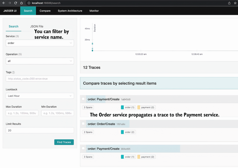
You can then access the Jaeger UI by visiting http://localhost:16686 in the browser, as shown in figure 9.10.
The tracing search screen is a simple interface that allows you to search for traces and see more details by clicking on the spans. In figure 9.11, you can see examples in which the Order service has one span and the Payment service two spans. Let’s look at how we can use those details to understand service metrics.
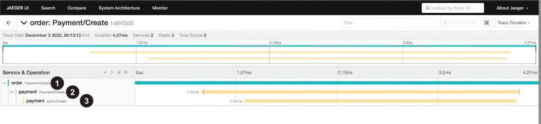
The request generates traces and spans while it visits each service, and those spans contain useful metrics about services. With the tracing provider’s help, we can ship those traces and metrics to collector endpoints in the Jaeger ecosystem. We already checked a very basic example in the previous section, and now we will review a specific trace to understand what is going on in it. From the Jaeger UI (figure 9.10), we will see the details in figure 9.11 after clicking the first trace.
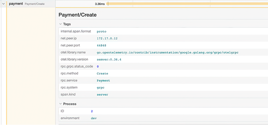
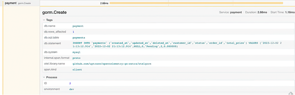
In figure 9.11, it took 4.2 ms to finish the create order flow. The Payment Create operation in the Payment service took 3.36 ms, which contains a DB-related operation that took 2.88 ms. Hopefully, since we are using GORM in our project and the OpenTelemetry registry already has GORM instrumentation, we can collect metrics from DB-related operations. We can also see more details by clicking any of those spans. For example, payment/PaymentCreate has the information shown in figure 9.12.
As you can see, there is plenty of metadata in span details, and rpc.service was defined in our tracing provider, as well as the ID and environment. (You can see the description of the fields in figure 9.12 here: http://mng.bz/9DY0.) span.kind was also defined, which shows us this is a server-related metric. Let’s look at another example.
In a DB operation, you can see database, statement, and so on. These metrics are helpful to spot the root cause of a problem, as the provided SQL statement can provide a lot of information, such as the performance of the query. You can check traces, spans, and related metrics, as well as the performance summary of gRPC microservices using the Jaeger service performance monitoring (SPM) component (figure 9.13).
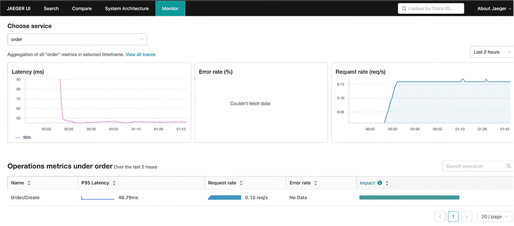
In SPM, you can see the performance monitoring metrics for each service after clicking the Monitor menu in Jaeger UI. To understand the basic performance analysis of the Order service, select Order in the dropdown menu to see a performance summary that contains p95 latency, request rate, error rate, and so on (figure 9.14).
In figure 9.14, the p95 latency of the Order service is 46.79 ms, meaning 95% of the latencies are 46.79 ms or less. You can also see the frequency of the requests: 6 per second. As a reminder, these performance metrics are aggregated from Prometheus. Now that we have checked traces and metrics, let’s look at how we can handle logs in Kubernetes.
Application logs are important to reference when we have a problem in the live environment because they contain messages from the application that can help us understand what happened. Analyzing logs may become more challenging in a distributed system like gRPC microservices because we need to see the logs in a meaningful order. In a logging backend system, you can see logs from different services and from different systems. If we want to filter for only the logs in an operation, we need a filter field that belongs to that operation. I have seen this with different names, such as “correlation ID” and “distributed trace ID,” which refer to the tracing ID we saw in OpenTelemetry. Let’s look at how to inject this trace ID into our application logs to filter logs by trace IDs.
Plenty of logging libraries exist in the Go ecosystem, but we will use logrus (https://github.com/sirupsen/logrus) in our examples. Here’s a simple example:
log.WithFields(log.Fields{
    "id": “12212”
  }).Info("Order is updated")
After using this code, a message with metadata and key-value pairs is provided in standard output. In this example, order ID metadata is inside a log message, so if you ship this message to the logging backend, you can filter logs using that metadata.
Let’s go back to distributed systems. To inject trace and span IDs into every log we printed using the logrus library, we can configure it to use a log formatter:
...
type serviceLogger struct {
    formatter log.JSONFormatter                                    ❶
}

func (l serviceLogger) Format(entry *log.Entry) ([]byte, error) {
    span := trace.SpanFromContext(entry.Context)                   ❷
    entry.Data["trace_id"] = span.SpanContext().TraceID().String()
    entry.Data["span_id"] = span.SpanContext().SpanID().String()
    //Below injection is Just to understand what Context has
    entry.Data["Context"] = span.SpanContext()
    return l.formatter.Format(entry)                               ❸
}
...
❶ Logs will be printed in JSON format.
❷ Gets the span from the context
❸ Injects the trace and span into the current log message
This is just a definition of a log formatter, and when you look at the logic in the Format function, you can see it loads span data from context and configures the existing log entry to inject tracing data. How is this log formatter used? There are multiple answers to this question: you can pass this formatter to other packages to use it, or maybe put formatter initialization in the init() function to configure log formatting once the main.go is loaded:
func init() {                                                   ❶
    log.SetFormatter(serviceLogger{                             ❷
        formatter: log.JSONFormatter{FieldMap: log.FieldMap{    ❸
            "msg": "message",
        }},
    })
    log.SetOutput(os.Stdout)                                    ❹
    log.SetLevel(log.InfoLevel)                                 ❺
}
❶ Executes the function on the file load
❷ Sets serviceLogger as the log formatter
❹ Logs are printed in standard output.
Log formatters can be added to the cmd/main.go file, and once you add the init() function it, the log formatter will be initialized when the application starts. Then, you can use logrus in any location, and it will use that formatter globally in your project:
log.WithContext(ctx).Info("Creating order...")
If you make a gRPC call to CreateOrder, logrus will use the context to populate its content, which you can see in trace and span information:
{"Context":{"TraceID":"4a55375c835c1e0f78d5a0001b6f5f5d","SpanID":"1ab65b1c
➥ 982ee940","TraceFlags":"01","TraceState":"","Remote":false},"level":"in
➥ fo","message":"Creatingorder...","span_id":"1ab65b1c982ee940","time":"2
➥ 022-12-04T06:37:25Z","trace_id":"4a55375c835c1e0f78d5a0001b6f5f5d"}
TraceID and SpanID fields can be used in the logging backend to filter and show the logs related to a specific operation. However, how can we get the TraceID to complete a filter operation? In gRPC, we use context to propagate tracing information between services, which can be injected into the response context so that we can use it.
As you can see in the example, the logs are in JSON format, and you may think this is hard to read in the standard output. However, this usage is very useful for logging backends because they can easily map JSON fields into search fields, which you can use while searching. If you use plain text logs, you need to develop a proper parser to help the logging agent or backend convert log messages into a more readable data structure. Now that we also understand how to inject tracing information into application logs, let’s look at how we can collect logs from those applications.
You can get Kubernetes pod logs in the terminal with the following command:
kubectl logs -f order-74b6b997c-4rwb5
kubectl is not magic here, as whatever you write in the logs in standard output is stored in a log file in the file system. These log files have a naming convention, such as <pod>_<namespace>_<container>-<unique_identifier>.log, and are located in /var/log/ containers in Kubernetes nodes. The post is that collecting logs is not that difficult; a simple agent could stream those files and process them. A typical log collection setup needs one log collection agent per Kubernetes node to reach the log files under /var/log/containers.
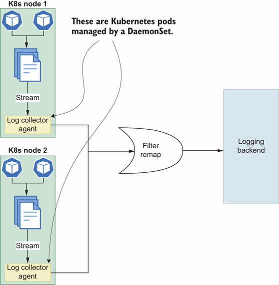
Figure 9.15 shows a log collector agent in every Kubernetes node that streams log files generated by the containers inside pods. These collector agents are mostly Kubernetes pods, and Kubernetes DaemonSets manage them to ensure there is one running process on each node, which allows you to access logs separately.
We will use Fluent Bit (https://fluentbit.io/), an open source logs and metrics processor and shipper in a cloud-native environment, as a log collector agent. We can use Helm Charts to install Fluent Bit in the Kubernetes environment:
helm repo add fluent https://fluent.github.io/helm-charts
helm repo update
helm install fluent-bit fluent/fluent-bit
This will create a Kubernetes DaemonSet, which spins up a pod per Kubernetes node to collect logs. By default, it tries to connect Elasticsearch with the domain name elasticsearch-master, which means we must configure it via values.yaml. Before modifying values.yaml, let’s look at how to use Elasticsearch and Kibana to make logs more accessible.
Elasticsearch is a powerful search engine based on Lucene (https://lucene.apache.org/core/). There are several options for using Elasticsearch, such as in AWS, GCP, Azure Marketplace, or Elastic Cloud (https://www.elastic.co/). To better understand the logic, let’s try to install Elasticsearch in our local Kubernetes cluster by installing CRDs dedicated to Elasticsearch components and installing the operator to create an Elasticsearch cluster:
kubectl create -f https://download.elastic.co/downloads/eck/2.5.0/crds.yaml
Since CRDs are available in Kubernetes, let’s install the operator as follows.
kubectl apply -f https://download.elastic.co/downloads/eck/2.5.0/operator.yaml
Now that the CRDs and the operator are ready to handle the lifecycle of the Elasticsearch cluster, let’s send an Elasticsearch cluster creation request:
cat <<EOF | kubectl apply -f -
apiVersion: elasticsearch.k8s.elastic.co/v1   ❶
kind: Elasticsearch
metadata:
  name: quickstart
spec:
  version: 8.5.2
  nodeSets:
  - name: default
    count: 1
    config:
      node.store.allow_mmap: false            ❷
EOF
To avoid disturbing the context, I will not dive deeply into an Elasticsearch-specific configuration, but you can read about virtual memory configuration (http://mng.bz/jPpV), which is used in this example. The previous command will apply the Elasticsearch spec to the Kubernetes cluster, which ends up deploying an Elasticsearch instance. Now we can configure Fluent Bit, but we need one more thing from Elasticsearch: a password. You can use the following command in your terminal to get a password:
PASSWORD=$(kubectl get secret quickstart-es-elastic-user -o go-
➥ template='{{.data.elastic | base64decode}}')
This simply gets the secret value for elastic and decodes it so that you can reach it via $PASSWORD variable.
In Fluent Bit, we can focus on the config in values.yaml, especially the outputs section, which defines output destinations so that Fluent Bit can forward the logs to them. To achieve that, let’s create a fluent.yaml file in the root of the microservices project and add the following config:
config:
  outputs: |
    [OUTPUT]
        Name es
        Match kube.*                 ❶
        Host quickstart-es-http      ❷
        HTTP_User elastic            ❸
        HTTP_Password $PASSWORD      ❹
        tls On
        tls.verify Off               ❺
        Logstash_Format On
        Retry_Limit False
❶ Forward log that matches kube
To provide more context for the config, the values we provided in the Host, HTTP_User, and HTTP_Passwd fields are all generated by Elasticsearch deployments. If you have an existing Elasticsearch cluster, you must provide your settings. By default, TLS is enabled for the client-elasticsearch connection, but since this is a local deployment, TLS verification is disabled. We also defined the log format as Logstash (https://www.elastic.co/logstash/) and removed the limitation of the retry operation. If Fluent Bit fails on log forwarding to Elasticsearch, it will retry infinitely. As a final step, let’s update the Fluent Bit Helm Chart:
helm upgrade --install fluent-bit fluent/fluent-bit -f fluent.yaml
Our application is running, the Elasticsearch logging backend is running, and Fluent Bit forwards logs to Elasticsearch. What about visualization? Let’s look at how we can visualize our logs in the Kubernetes environment.
Kibana (https://www.elastic.co/kibana/) is a data visualization dashboard for Elasticsearch. This UI application uses Elasticsearch as an API backend to aggregate a search dashboard. We installed CRDs in the previous section, which contain Kibana-related resources. To install Kibana in Kubernetes, you can apply a Kibana resource:
cat <<EOF | kubectl apply -f -
apiVersion: kibana.k8s.elastic.co/v1   ❶
kind: Kibana
metadata:
  name: quickstart
spec:
  version: 8.5.2
  count: 1
  elasticsearchRef:
    name: quickstart                   ❷
EOF
❷ Reference to Elasticsearch backend
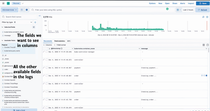
This will simply deploy Kibana, and you can access it via port forwarding to port 5601, the default port for Kibana. When you go to http://localhost:5601 in your browser, you may get a warning about defining the index. In that case, you can provide an arbitrary name and an index pattern (e.g., log*), which simply matches Logstash logs. Figure 9.16 shows the dashboard with Kubernetes logs.
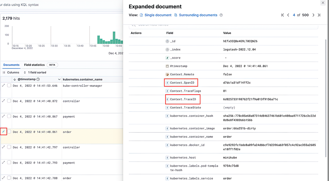
As shown in figure 9.16, I selected only the container name and message fields. All the available fields are processed and shipped to Elasticsearch by Fluent Bit, which means you can modify the syntax in the Fluent Bit configuration based on your needs. If you click any logs there, you can see more details, as shown in figure 9.17.
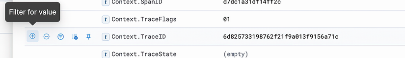
Since TraceID and SpanID are already injected into application logs, we can see them in the Kibana dashboard. To see all the logs under a specific TraceID, you can do a search (figure 9.18).
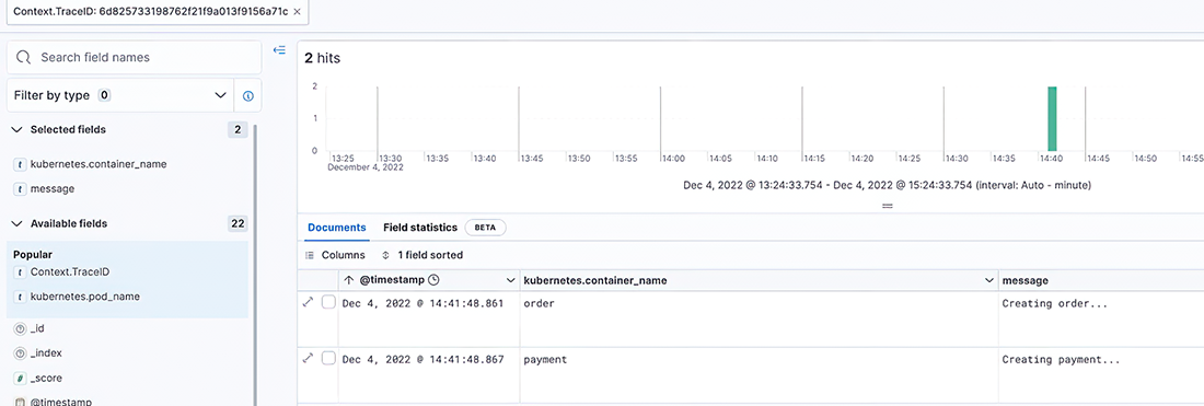
You can see that the entire flow belongs to a specific TraceID (figure 9.19).
Observability is key to successful, stress-free, and more visible microservices.
The main components for observability are traces, metrics, and logs, and correlating them is important, as it allows you to detect why an application is slow, what the metrics are, and what the related logs are at the time a metrics anomaly is detected.
Traces are important for understanding request flows in a microservices environment, especially if they have related metrics instrumented by OpenTelemetry SDKs.
A cluster-level logging architecture with Fluent Bit as a collector, Elasticsearch as a logging backend, and Kibana as data visualization increases microservices’ observability. This setup provides flexibility for searching structured log data.